Prepared to invest in an Up-and-Down Market February 21, 2013

On Friday, the S&P 500 was up about 7% from the start of the year. This is very similar to the gains through mid-February in 2011 and 2012. These steady gains then began to be revealed as the first stage of a volatile year that frequently exhibited 5 – 15% swings in the stock market, as you can see in Figure 1.

Again in 2013, the stock market may post a gain, but those gains may be hard to discern during the course of a year that exhibits frequent swings of 5 – 15%. Fortunately, this volatility is perfectly normal.

The investing environment may be like that of 1994 and 2004, the last two times the economy experienced a transition in Federal Reserve (Fed) policy. Both 1994 and 2004 had multiple 5 – 15% pullbacks in the S&P 500 as the recovery matured, stimulus faded, and the Fed hiked interest rates marking a return to normal conditions. Both years also provided only single-digit buy-and-hold returns. Yet neither year marked the end of the bull market.

Just as in 1994 and 2004, market participants are likely to remain focused on the Fed over the coming two weeks. First, this week the Fed releases the minutes to their January meeting, providing more detail on the deliberations. Second, next week (February 26 – 27) Fed Chairman Ben Bernanke will deliver his semi-annual report on the economy and interest rates to House and Senate panels.

A key contributor to the volatility in 1994 and 2004 was the normalization of monetary policy — or, in other words, hikes to the federal funds rate by the Fed. The volatility began early in those years as the Fed signaled the coming of the rate hikes that took place later in the year. While a rate hike remains a year or two away at the earliest, the Fed is likely to begin to slow or stop the current bond-buying program, known as quantitative easing, later this year or very early in 2014. The Fed will likely note that this change in policy marks a “normalization” after providing exceptional liquidity since late 2008. Regardless of the Fed’s description, these steps toward a return to a more normal monetary environment are likely to lead to higher interest rates and tighter credit conditions for borrowers, even without the hikes to the federal funds rate that can weigh on the stock market.

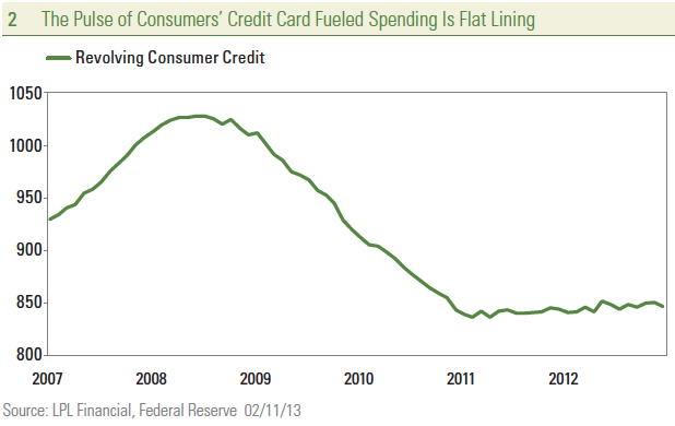
Changes to Fed programs — or even deliberations months ahead of the potential end of a program or start of a new one — have punctuated the volatile moves in the market over the past five years, as you can see in Figure 2. The coming weeks could begin to reintroduce some Fed-related volatility to the markets if the Fed signals any potential upcoming actions. However, pronounced moves are more likely to come later in the year as the Fed is closer to a change in policy.

It is relatively easy to figure out how to invest when you believe the market is likely to go up or go down, but how do you invest when it is likely to go both up AND down? There are several potential ways to benefit from market volatility, including:

• Rebalance tactically – More frequent rebalancing and tactical adjustments to portfolios are recommended to take advantage of the opportunities created by the pullbacks and rallies. Seeking undervalued opportunities and taking profits are key elements of a successful volatility strategy.
• Seek yield – Focusing on the yield of an investment rather than solely on price appreciation can help enhance total returns. Bank loans and even alternative vehicles like master limited partnerships (MLPs) offer a potential yield advantage over investments that are solely price-driven during periods of high volatility.
• Go active – Using active management rather than passive indexing strategies to enhance returns. In general, active managers tend to outperform their indexes when volatility rises, according to LPL Financial Research analysis. Opportunistic-style investments provide a wide range of opportunities for managers to exploit during volatile markets.
• Think alternatively – Increase diversification by adding low-correlation investments and incorporating non-traditional strategies that aim to provide downside protection, risk management, and may benefit from an environment of increased volatility. This would include exposure to covered calls, managed futures, global macro, long/short, market neutral, and absolute return strategies.

Some investors are wary of this volatility and view it as a sign of a fragile market. We see volatility as a normal, and even potentially rewarding, part of the investing environment for those who know how to invest for volatility.

________________________________________________________________________________________

IMPORTANT DISCLOSURES

The opinions voiced in this material are for general information only and are not intended to provide specific advice or recommendations for any individual. To determine which investment(s) may be appropriate for you, consult your financial advisor prior to investing. All performance reference is historical and is no guarantee of future results. All indices are unmanaged and cannot be invested into directly.

Stock investing involves risk, including the risk of loss.

Correlation is a statistical measure of how two securities move in relation to each other. Correlations are used in advanced portfolio management.

Quantitative easing is a government monetary policy occasionally used to increase the money supply by buying government securities or other securities from the market. Quantitative easing increases the money supply by flooding financial institutions with capital in an effort to promote increased lending and liquidity.

Bank loans are loans issued by below investment-grade companies for short-term funding purposes with higher yield than short-term debt and involve risk.

Master limited partnership (MLP) is a type of limited partnership that is publicly traded. There are two types of partners in this type of partnership: The limited partner is the person or group that provides the capital to the MLP and receives periodic income distributions from the MLP’s cash flow, whereas the general partner is the party responsible for managing the MLP’s affairs and receives compensation that is linked to the performance of the venture.

Federal Funds Rate is the interest rate at which a depository institution lends immediately available funds (balances at the Federal Reserve) to another depository institution overnight.

Operation Twist is the name given to a Federal Reserve monetary policy operation that involves the purchase and sale of bonds. “Operation Twist” describes a monetary process where the Fed buys and sells short-term and long-term bonds depending on their objective.

Yield is the income return on an investment. This refers to the interest or dividends received from a security and is usually expressed annually as a percentage based on the investment’s cost, its current market value or its face value.

Alternative investments may not be suitable for all investors and involve special risks such as leveraging the investment, potential adverse market forces, regulatory changes and potentially illiquidity. The strategies employed in the management of alternative investments may accelerate the velocity of potential losses.

There is no guarantee that a diversified portfolio will enhance overall returns or outperform a non-diversified portfolio. Diversification does not protect against market risk.

________________________________________________________________________________________

INDEX DEFINITIONS

The Standard & Poor’s 500 Index is a capitalization-weighted index of 500 stocks designed to measure performance of the broad domestic economy through changes in the aggregate market value of 500 stocks representing all major industries.

________________________________________________________________________________________

 This research material has been prepared by LPL Financial.

To the extent you are receiving investment advice from a separately registered independent investment advisor, please note that LPL Financial is not an affiliate of and makes no representation with respect to such entity.

Not FDIC or NCUA/NCUSIF Insured | No Bank or Credit Union Guarantee | May Lose Value | Not Guaranteed by any Government Agency | Not a Bank/Credit Union Deposit

Member FINRA/SIP

________________________________________________________________________________________

Stay Connected with Us!

    

www.garrettandrobinson.com

Residential Recovery – Weekly Economic Commentary February 15, 2013

Residential Recovery

Over the second half of February 2013, financial markets will begin to digest early 2013 data on the housing market: housing starts, home prices, new and existing home sales, and pending home sales. Housing made a splash in late January 2013, as the gross domestic product (GDP) data for 2012 revealed that housing added to GDP in 2012 for the first time since 2005. Market participants are now asking whether housing can continue to contribute to the economy in 2013 — and beyond.

In our view, the U.S. housing market is still in the early stage of recovering from the 2006-2009 bust that followed the decade-and-a-half (early 1990s through mid-2000s) housing boom that began to show severe cracks in 2007 and collapsed in 2008. The collapse in housing, in turn, was a major contributor to the financial crisis and Great Recession of 2007 – 2009. The housing market, along with many financial markets and global economies, are still feeling the after-effects of the housing collapse.

“Location, Location, Location”

 As the old saying goes, the real estate market is all about “location, location,location.” When we discuss the housing market, we do so from a national perspective: what is happening to the housing market on your street or in your neighborhood, town, city, or state may be completely different (better or worse) than what is happening nationwide. With that important caveat in mind, we can say that the housing market (sales, prices, construction, etc.) hit bottom in early 2009, and moved sideways between early 2009 and late 2011 before beginning to pick up momentum at the start of 2012. Until housing added 0.3 percentage points to overall GDP in 2012, housing construction (the most direct way housing impacts GDP) had not been a significant, sustained contributor to economic growth since 2005 (as measured by GDP). The lack of participation from housing has been one of the main reasons (along with the severe cutbacks in state and local governments) behind the sluggish economic recovery so far. Looking ahead through the remainder of 2013, we see housing making another significant (0.3 – 0.5 percentage points) contribution to GDP growth, as the positives driving the residential recovery more than outweigh the negatives. There are a number of direct (housing starts, housing sales, construction spending, home prices) and indirect (homebuilder sentiment, mortgage applications, foreclosures, inventories of unsold homes, mortgage rates, housing vacancies, lumber prices, prices of publicly traded homebuilders) ways to measure the health of the housing market. The U.S. government and private sources collect and disseminate these data. A quick recap of these various indicators is below.

Taking the Pulse of the Residential Recovery

• Record housing affordability. Housing affordability, the ability of a household with the median income to afford the payments on a median priced house at prevailing mortgage rates, is at an all-time high. Rising incomes, record-low mortgage rates, and the aftermath of the 20 – 30% drop in home prices nationwide between 2005 and 2009 account for the record level of affordability [Figure 1].
• Housing market improvement is broadening out. According to the National Association of Homebuilders Improving Market Index, in February 2013, 259 of 361 metropolitan areas across the United States are “improving,” reflecting six consecutive months of increasing employment, increasing home prices, and increasing housing permits. In February 2011, just 98 markets made the list [Figure 2].
• Homebuilder sentiment. At 47 (on a scale of 0 to 100, where zero is the worst and 100 is the best), the index of homebuilder sentiment has surged over the past 18 months and now sits at its highest level since mid-2006. However, during the peak of the housing boom, this index was as high as 70, and averaged 60. The private sector’s National Association of Home Builders compiles the homebuilder sentiment data.

• Inventories of unsold homes are low. Despite a lingering “shadow inventory,” defined as homes in or close to foreclosure, and homes still sitting on bank balance sheets, inventories of unsold existing homes are the lowest they have been since 2000/2001. The official count of the inventory of unsold single family existing homes (from the National Association of Realtors), along with the record-low inventory of new homes for sale, tells us that there are 1.7 million homes for sale. Depending on the data source cited (there is no “official” number for shadow inventory), the shadow inventory is in the 1.5 – 2.0 million range. While still well above average, the shadow inventory has moved sharply lower over the past 18 months [Figure 3].

• Housing starts and building permits. Responding to less demand for housing, difficult credit conditions, and a glut of unsold inventory, homebuilders drastically cut the number of new housing starts in recent years. Housing starts peaked at 2.3 million units in early 2006, and by early 2009 had dropped to under 500,000 units, an 80% drop. Since then, as inventories of unsold new and existing homes shrunk and the economy and financing conditions improved, starts have more than doubled, to nearly a 1 million annualized rate in late 2012. Still, despite the 100% move off the bottom, housing starts remain 60% below their all-time high. The U.S. Commerce Department collects housing starts and building permits (a key leading indicator of starts). Homebuilder stocks. Although they are not a perfect leading indicator of the health of the housing market, the S&P 500 homebuilders’ index has nearly tripled since October 2011. Despite that dramatic rally, homebuilding stocks — as measured by the S&P 500 homebuilders’ index — are still more than 50% below the peak hit in mid-2005.

• Lumber prices. Lumber is a key input to the homebuilding process. Lumber prices peaked in mid-2004 — a year or so before the housing market peaked — and declined by nearly 70% by early 2009. Since early 2009, lumber prices have nearly tripled (in fits and starts), but still remain more than 15% below their 2004 peak. Lumber prices are set in the open market and trade on several global commodity exchanges [Figure 4].
• Supply and demand for home mortgages. From the mid-1990s through late 2006, bank lending standards (down payment required, credit scores, work history, etc.) for residential mortgages were relatively easy. Coupled with low rates and rapid innovation in financial products backing residential mortgages, this easy credit helped to fuel the housing boom. The banking industry began tightening lending standards in early 2007, and continued to tighten for more than two years. Lending standards eased in 2009 and 2010, but remain more restrictive than they were in the true boom years from 2004 to 2006. On the demand side of the equation, consumer demand for mortgages remained muted during the first two-and-a-half years (early 2009 through late 2011) of the housing recovery, as consumers remained uncertain about prospects for home price appreciation and their own financial and labor market status. Since then, an improved labor market, Federal Reserve (Fed) actions to lower mortgage rates, and rising home prices have driven consumer demand for mortgages to levels not seen since the early 2000s. The Fed compiles these data in the Senior Loan Officer Survey, which is released quarterly. Low mortgage rates — thanks to a sluggish economy and aggressive Fed — are making housing an attractive alternative to renting. The housing recovery is dependent upon low interest rates, but not necessarily the lowest interest rates. History shows us that if job and income growth can rise along with mortgage rates, the growth in housing can continue.
• Mortgage applications. Measured by the private sector’s Mortgage Bankers Association, the volume of mortgage applications has doubled since late 2008, but remains well below its early- to mid-2000s peak. Applications for refinancing have tripled since late 2008. Weekly mortgage applications are a key gauge of consumer demand for housing. Mortgage applications are a component of our weekly Current Conditions Index.
• Foreclosure activity. After a de facto moratorium on new foreclosures was put into place in late 2010, as the U.S. and individual state governments sued mortgage processors and banks, the pace of new foreclosures slowed down. By early 2012, new foreclosures were at the lowest level since mid-2007. This legal action was settled in late 2011, and many housing market observers expected that the foreclosure pipeline would pick back up again. However, there was no discernible uptick in foreclosures after the moratorium was lifted, and the pipeline of new defaults and overall mortgage delinquencies continues to drain, aided by a better economy and job market. There are various public and private sources for foreclosure and delinquency data. On the private sector side, firms like RealtyTrak, Lender Processing Services, and the Mortgage Bankers Association provide data. Freddie Mac, Fannie Mae, and the Federal Housing Finance Administration (FHFA) are among the government agencies that compile data on delinquencies and foreclosures.
• Construction employment. As measured by the U.S. Department of Labor, employment in residential construction increased by more than 1 million between the early 2000s and 2006 to nearly 3.5 million workers. Since then, workers employed in the construction of new homes dropped by nearly 50%, bottoming out at just under 2 million in late 2010. Construction employment has since moved up modestly, adding just 50,000 jobs in 2011 and another 40,000 in 2012. Construction employment is poised to make a consistent contribution to overall employment in 2013, and may add as many as 10,000 – 20,000 jobs per month to overall employment.
• Construction put into place. The value of new residential construction put into place peaked at $525 billion in early 2006. Since then, construction of new homes has plummeted, and by mid-2009, just $122 billion in new home construction was underway. This data series moved sideways for about 18 months, hitting another low ($119 billion) in early 2011. Home construction has since increased by more than 40% to $170 billion, but new home construction is still running more than 70% below its peak. The U.S. Commerce Department collects these data.
• Home prices. Home prices are rising at the fastest pace since August 2006, with a 5.5% year-over-year gain according to the Case-Shiller home price data. Home prices are rising generally, but soaring in states like Phoenix and San Francisco while they continue to slump in New York and Chicago. About half of all U.S. distressed properties in the U.S. are concentrated in five states: New York, Illinois, Florida, California, and New Jersey. Builders are concentrating on those states where the demand is strongest. There are a variety of sources for home prices from both the private sector — Case-Shiller Home Price Index, CoreLogic, Zillow, RadarLogic, National Association of Realtors — and the U.S. government — Freddie Mac, Fannie Mae, Federal Housing Finance Agency, etc. In general, these indices all suggest that home prices fell by between 20% and 30% between mid-2005 and early 2009. Over the next two-and-a-half years, home prices moved sideways. Today, home prices have risen by between 5% and 15% from their cycle lows. Price changes before, during, and after the bubble vary widely by region, price of home, and type of property (single family versus condo, distressed, and non-distressed, etc.).

• Demand for housing. Unemployed new graduates were staying with their parents or renting in large groups rather than moving into homes of their own for years after the 2008 – 09 recession. But that is ending. Over the last year, “household formation” has been picking up. In fact, the number of net new formations on a rolling 12-month basis is back to levels last seen in 2006. Thanks to the echo boomers reaching their midto- late 20s. Most importantly, 2012 marked the second year in a row that housing formations (demand) outstripped housing completions (supply). Housing starts are headed consistently higher, boosting housing-related stocks. Although it has slowed from its pre-Great Recession pace, new household formation is running just under 1.0% per year [Figure 5]. By early 2011, the gap between new household (see nearby box) formation and new housing starts had never been wider. Soon thereafter, housing starts began to recover, and the healing in the housing market began to accelerate. However, there are still more than 18 million vacant homes — down from the peak of nearly 20 million, but still well above the pre-Great Recession level of 14 – 15 million. The U.S. Census Bureau collects the data on household formation and housing vacancies.

On balance, most evidence suggests that the housing market has picked up momentum over the past year or so, after struggling for three years since hitting rock bottom in early 2009. The pace (and sustainability) of the nascent housing recovery will help to determine the pace of the overall economic recovery. We expect housing to make a positive contribution to overall GDP growth in 2013, but that it will still take several more years before the national housing market is back to normal.

________________________________________________________________________________________

IMPORTANT DISCLOSURES

The opinions voiced in this material are for general information only and are not intended to provide specific advice or recommendations for any individual. To determine which investment(s) may be appropriate for you, consult your financial advisor prior to investing. All performance reference is historical and is no guarantee of future results. All indices are unmanaged and cannot be invested into directly.

Gross Domestic Product (GDP) is the monetary value of all the finished goods and services produced within a country’s borders in a specific time period, though GDP is usually calculated on an annual basis. It includes all of private and public consumption, government outlays, investments and exports less imports that occur within a defined territory.

The economic forecasts set forth in the presentation may not develop as predicted and there can be no guarantee that strategies promoted will be successful.

Stock investing involves risk including loss of principal.

The Federal Open Market Committee (FOMC), a committee within the Federal Reserve System, is charged under the United States law with overseeing the nation’s open market operations (i.e., the Fed’s buying and selling of United States Treasure securities).

________________________________________________________________________________________

INDEX DESCRIPTIONS

The Chicago Area Purchasing Manager Index that is read on a monthly basis to gauge how manufacturing activity is performing. This index is a true snapshot of how manufacturing and corresponding businesses are performing for a given month. A reading of 50 or above is considered a positive reading. Anything below 50

is considered to indicate a decline in activity. Readings of the index have the ability to shift the day’s trading session one way or another based on the results.

The National Association of Home Builders (NAHB)/First American Improving Markets Index measures the number of housing markets that are showing signs of improving economic health each month. The metro areas which see growth in employment, house prices, and single family housing at least six months after

each indicator’s respective trough, are categorized as improving and included in the index.

The S&P/Case-Shiller U.S. National Home Price Index measures the change in value of the U.S. residential housing market. The S&P/Chase-Shiller U.S. National Home Price Index tracks the growth in value of real estate by following the purchase price and resale value of homes that have undergone a minimum of two arm’s-length transactions. The index is named for its creators, Karl Chase and Robert Shiller.

The Standard and Poor’s 500 Homebuilding Index is a capitalization-weighted index. The index was developed with a base level of 10 for the 1941-43 base period, the parent index is SPX.

The Empire State Manufacturing Index is a seasonally-adjusted index that tracks the results of the Empire State Manufacturing Survey. The survey is distributed to roughly 175 manufacturing executives and asks questions intended to gauge both the current sentiment of the executives and their six-month outlook on the sector.

_______________________________________________________________________________________

This research material has been prepared by LPL Financial.

To the extent you are receiving investment advice from a separately registered independent investment advisor, please note that LPL Financial is

not an affiliate of and makes no representation with respect to such entity.

Not FDIC/NCUA Insured | Not Bank/Credit Union Guaranteed | May Lose Value | Not Guaranteed by any Government Agency | Not a Bank/Credit Union Deposit

 _______________________________________________________________________________________

Member FINRA/SIPC

Page 6 of 6

RES 4080 0213

Tracking #1-141283 (Exp. 02/14)

Investor’s Guide to the State of the Union Address February 12, 2013

Investor’s Guide to the State of the Union Address

President Obama’s State of the Union (SOTU), scheduled for Tuesday, February 12, is unlikely to be a big market mover. In fact, most SOTU speeches see less than a 1% move in the stock market on the following day, and the average move is only 0.15% [Figure 1].

In his SOTU address on Tuesday, President Obama will present key themes that may impact certain industries and asset classes. While gun control and immigration will likely comprise important themes, they have minor market impact. The two major themes that we will be listening for with potential to impact the markets are: the fiscal cliff and energy independence.

Fiscal Cliff Part II

Early in his speech, the President will be forced to talk about the fiscal cliff part II. There are three remaining components to the fiscal cliff that are yet to be resolved: the sequester taking effect March 1, the government shutdown set for March 27, and the debt ceiling to be hit on May 19.

• The President will likely restate his recent comments about replacing the spending cuts that kick in on March 1, known as the sequester, with some combination of tax increases and spending cuts. However, this has little chance of passing the House after Republicans supported tax increases in the first fiscal cliff deal. The Congressional Budget Office estimates that the fiscal drag from the sequester in 2013 would be about $85 billion, or about 0.5% of gross domestic product (GDP.) This adds to the roughly 1.5% drag on the economy from the fiscal cliff tax increases that went into place January 1. That is a materially negative impact for an economy that registered a contraction in the fourth quarter and is on track for only sluggish growth in the current quarter.

Comments that suggest the President is open to mitigating the defense cuts in exchange for cuts elsewhere, rather than tax increases, may be a positive for the markets — especially for stocks in the defense industry, which have been pulling back lately as the cuts have loomed. Unless changed, defense spending (other than for military personnel) will be cut by around 8% across the board, while nondefense funding that is subject to the automatic reductions will be cut by between 5% and 6%.

• The continuing resolution funding the government expires on March 27 and could prompt a government shutdown (though certain essential components like the armed forces will continue to operate). While tax collections will be reaching their seasonal peak as the April 15 deadline approaches, tax refunds processed by the IRS may take much longer than usual and could cause consumer spending to drop and negatively impact stocks in the consumer discretionary sector. In 2012, the average tax refund check was nearly $3,000, all together totaling $175 billion. The drag on incomes could be felt since consumers have lacked the confidence to fund spending with credit cards in recent years [Figure 2]. During the previous two government shutdowns, it was short-lived. It lasted five days in November 1995 and was followed by 21 days in January 1996. As long as talks are proceeding, we expect another continuing resolution to be passed to fund the government for a few more months or until September 30 to avoid a lengthy shutdown.

• While the debt ceiling has been pushed back to May 19, it will soon be upon us again. If no further action is taken before May 19, the Treasury will once again resort to extraordinary measures to allow the government to continue operating. As precursor to restating these negotiations, President Obama will likely talk about a “balanced package” of spending cuts and tax increases to reduce the deficit and need for additional borrowing. With the potential for additional tax rate increases on the horizon, high dividend-paying stocks and municipal bonds (given the potential elimination of some deductions) could react negatively, which may present a buying opportunity.

These fiscal cliff issues leave little likelihood that other recurring themes in the President’s SOTU address see any legislative action that otherwise could impact certain asset classes. For example, the President is likely to again tout the need for greater infrastructure investment — a potential positive for some stocks in the industrial and materials sectors were it to actually take place. Another example is a new program to modify underwater mortgages that could act as a negative for mortgage-backed securities, if implemented.

Energy Independence

The President is likely to highlight the need for U.S. energy independence, noting the increasing domestic oil and gas production and voicing his continued support for sources of clean energy. Given their dependence on federal support programs, the stocks of producers of wind, solar, and other clean energy sources often tend to be volatile around the SOTU addresses in recent years — sometimes seeing a big bounce that soon fades.

Regarding traditional sources of energy, investors are unlikely to hear anything on natural gas or coal that may turn around slumping coal stocks, but probably nothing that would accelerate their decline either. However, the President will likely highlight energy tax incentives for elimination known as the “percentage depletion allowance” and “expensing of intangible drilling costs.” These incentives exist to encourage small companies to produce oil from marginal wells that become profitable with the tax breaks. These marginal wells are old or small wells that do not produce much oil individually, but in total constitute most of the U.S.’s domestic oil and gas production. The percentage depletion allowance was eliminated in 1975 for the major oil companies, and their ability to expense intangible drilling costs expensing is very limited. Therefore, the potential elimination of these tax breaks would be unlikely to have a major negative effect on the major companies in the energy sector. However, the exploration and production industry of the energy sector could be negatively impacted, were these incentives to be eliminated, which we doubt will happen in 2013.

________________________________________________________________________________________

­­­­­­­­­­­­­­­­­­

IMPORTANT DISCLOSURES

The opinions voiced in this material are for general information only and are not intended to provide specific advice or recommendations for any individual. To determine which investment(s) may be appropriate for you, consult your financial advisor prior to investing. All performance reference is historical and is no guarantee of future results. All indices are unmanaged and cannot be invested into directly.

The economic forecasts set forth in the presentation may not develop as predicted and there can be no guarantee that strategies promoted will be successful.

Stock investing involves risk including loss of principal.

The commentary expresses the political view of the author and in no way represents the views of LPL Financial. The assumptions made are based upon approvals by Congress and are subject to change. While individual advisors and investors may of course have their own personal views or preferences when it comes to matters of public and political policy, the author is trying to provide insights from the available data, allowing readers to make fully informed decisions.

Municipal bonds are subject to availability and change in price. They are subject to market and interest rate risk if sold prior to maturity. Bond values will decline as interest rates rise. Interest income may be subject to the alternative minimum tax. Municipal bonds are federally tax-free but other state and local taxes may apply.

Mortgage-Backed Security (MBS) is a type of asset-backed security that is secured by a mortgage or collection of mortgages. These securities must also be grouped in one of the top two ratings as determined by a accredited credit rating agency, and usually pay periodic payments that are similar to coupon payments. Furthermore, the mortgage must have originated from a regulated and authorized financial institution.

Mortgage-Backed Securities are subject to credit, default risk, prepayment risk that acts much like call risk when you get your principal back sooner than the stated maturity, extension risk, the opposite of prepayment risk, and interest rate risk.

Investments in specialized industry sectors have additional risk such as credit, regulatory, operational, business, economic and political risk which should carefully be considered before investing.

Consumer Discretionary Sector: Companies that tend to be the most sensitive to economic cycles. Its manufacturing segment includes automotive, household durable goods, textiles and apparel, and leisure equipment. The service segment includes hotels, restaurants and other leisure facilities, media production and services, consumer retailing and services and education services.

Energy Sector: Companies whose businesses are dominated by either of the following activities: The construction or provision of oil rigs, drilling equipment and other energy-related service and equipment, including seismic data collection. The exploration, production, marketing, refining and/or transportation of oil and gas products, coal and consumable fuels.

Industrials Sector: Companies whose businesses manufacture and distribute capital goods, including aerospace and defense, construction, engineering and building products, electrical equipment and industrial machinery. Also, companies that provide commercial services and supplies, including printing, employment, environmental and office services, or provide transportation services, including airlines, couriers, marine, road and rail, and transportation infrastructure.

Materials Sector: Companies that are engaged in a wide range of commodity-related manufacturing. Included in this sector are companies that manufacture chemicals, construction materials, glass, paper, forest products and related packaging products, metals, minerals and mining companies, including producers of steel.

________________________________________________________________________________________

INDEX DEFINITIONS

The Standard & Poor’s 500 Index is a capitalization-weighted index of 500 stocks designed to measure performance of the broad domestic economy through changes in the aggregate market value of 500 stocks representing all major industries.

This research material has been prepared by LPL Financial.

To the extent you are receiving investment advice from a separately registered independent investment advisor, please note that LPL Financial is not an affiliate of and makes no representation with respect to such entity.

Not FDIC or NCUA/NCUSIF Insured | No Bank or Credit Union Guarantee | May Lose Value | Not Guaranteed by any Government Agency | Not a Bank/Credit Union Deposit

Member FINRA/SIPC

Page 4 of 4

RES 4079 0213

Tracking #1-141165 (Exp. 02/14)

________________________________________________________________________________________

Stay Connected with Us!

    

www.garrettandrobinson.com

Less Defense? Weekly Economic Commentary February 7, 2013

Less Defense?

 On Sunday, February 3, 2013, the Baltimore Ravens defeated the San Francisco Forty Niners 34 – 31 to win Super Bowl XLVII. The talk of the game was certainly not about defense, but defense spending, and its impact on the economy, was a key topic of conversation in financial markets in the week leading up to the Super Bowl.

Economic Data Halftime Show Highlights

The financial markets in the week preceding the Super Bowl (January 28 – February 1) featured four key economic events;

• The Institute for Supply Management’s (ISM) Report on Business for January 2013;
•  The January 2013 employment report;
• The fourth quarter 2012 gross domestic product (GDP) report; and
• The Federal Reserve’s Federal Open Market (FOMC) meeting.

Any one of these events happening in one week would draw a great deal of attention from the media and financial market participants, but all of these top-ranked data points playing out in one week is rare — almost as rare as a power outage at the Super Bowl!

On balance, last week’s economic reports, along with the statement accompanying the FOMC meeting, revealed an economic playbook that included economic growth fast enough to create jobs and move the widely watched ISM index, at 53.1, to a nine-month high, but not fast enough to cause the Federal Reserve (Fed) to think about ending its program of bond purchases (quantitative easing, or QE3) anytime soon.

Last week’s economic data halftime show that drew the most attention was Thursday (January 31, 2013) morning’s release of the surprising -0.1% drop in GDP between the third and fourth quarters of 2012. Economists had been expecting a number around 1%. Within that surprisingly weak report was a stunning 22% drop in defense spending, the largest quarter-over-quarter drop in defense spending since 1972, as the Vietnam War was winding down. This drop alone shaved 1.3 percentage points from GDP. Although there is no precise measurement, the effect of Superstorm Sandy likely shaved another 0.5 percentage points off of GDP. Add in the 1.3 percentage point drag from fewer inventories being built up in the fourth quarter than in the third, and it is likely that real GDP growth would have been closer to 3.0% than to zero.

The drawdown in inventories may have been related to uncertainties among businesses ahead of the fiscal cliff and the impact of Superstorm Sandy. These are likely to be at least partially reversed in the first quarter of 2013 and add to GDP growth. However, the outlook for defense spending is a bit less certain due, in part, to yet another piece of the fiscal cliff: spending cuts known as sequestration.

Defense Spending Running at About 4 – 5% of GDP

At least a portion of the 22% drop in defense spending — from an annualized pace of $698.1 billion in the third quarter of 2012 to an annualized pace of $655.7 billion in the fourth quarter of 2012 — was likely due to the fiscal cliff, as some defense contractors may have curtailed some non-mission critical spending ahead of the pending cuts tied to sequestration. Indeed, the research and development-related portion of defense spending fell at a whopping 58% annualized rate in the fourth quarter, while outlays for troop pay dropped by just 3.0%. Thus, the ongoing drawdown in troop levels in Iraq and Afghanistan also most likely played only a part in the big drop in defense outlays in the fourth quarter. Government spending on big ticket military items like aircraft, missiles, ships, vehicles, and electronics fell by only 2.2% between the third and fourth quarters of 2012.

Between $25 billion and $30 billion of automatic spending cuts will hit defense spending on February 28, 2013, representing roughly a 10% cut to defense outlays, unless Congress acts to modify, suspend, or delay the cuts. Moving past the sequestration, the defense sector remains one of the largest single segments of the federal budget. In fiscal year 2012, defense spending was close to $640 billion and is one of the largest categories of discretionary spending. In recent years, defense spending has accounted for between 50% and 55% of discretionary spending, 4.5% of gross domestic product (GDP), and about 20% of overall federal government outlays. During the Reagan administration at the end of the Cold War, defense spending accounted for 65% of total discretionary spending, 6% of GDP, and nearly 30% of all federal government outlays. After the fall of

the Berlin Wall in 1989, defense spending as a percent of discretionary spending fell swiftly — bottoming out in 2001 at under 48%, 3% of GDP, and 15% of total federal outlays — just as the war on terror and the wars in Afghanistan and Iraq began.

Defense spending is often discussed as an area to cut in order to reduce the long-term deficit because it is such a large part of federal outlays. While there is likely some kernel of truth in oft-cited media reports of $600 hammers and $300 toilet seats being purchased by the Pentagon, eliminating all “waste, fraud, and abuse” from the defense budget, while a worthwhile endeavor, would only make a small dent in overall spending.

 

Potential Slowing in Pace of Defense Spending Ahead

Looking ahead from a budget perspective, perhaps the best that can be hoped for is a slowing in the pace of defense spending, not outright declines similar to those seen in the late 1970s and 1990s Some of the proposals put forth by the deficit commissions and the Congressional Budget Office (CBO) regarding defense spending include: 

• Freezing defense spending at current levels of GDP;
• Cutting the rate of increase in defense spending; and
• Finding savings within the Department of Defense’s procurement system.

 Please see our Weekly Economic Commentary: Budget Defense from November 26, 2012 for more details.

From a GDP perspective, the best case for defense spending in 2013 is that it has a modest positive impact on GDP. More likely, defense spending, after a rebound in the first quarter of 2013 on the heels of the big drop in the fourth quarter of 2012, is likely to be flat. The worst case — again from a GDP perspective — and least likely, would be if Congress can agree to substantial cuts to defense spending as part of an overall budget deal. In this scenario, defense would likely be a modest 0.1 to 0.2% drag on overall GDP growth in 2013 and beyond.

_______________________________________________________________________________

IMPORTANT DISCLOSURES

The opinions voiced in this material are for general information only and are not intended to provide specific advice or recommendations for any individual. To determine which investment(s) may be appropriate for you, consult your financial advisor prior to investing. All performance reference is historical and is no guarantee of future results. All indices are unmanaged and cannot be invested into directly.

Gross Domestic Product (GDP) is the monetary value of all the finished goods and services produced within a country’s borders in a specific time period, though GDP is usually calculated on an annual basis. It includes all of private and public consumption, government outlays, investments and exports less imports that occur within a defined territory.

The economic forecasts set forth in the presentation may not develop as predicted and there can be no guarantee that strategies promoted will be successful.

Stock investing involves risk including loss of principal.

International investing involves special risks, such as currency fluctuation and political instability, and may not be suitable for all investors.

The Federal Open Market Committee action known as Operation Twist began in 1961. The intent was to flatten the yield curve in order to promote capital inflows and strengthen the dollar. The Fed utilized open market operations to shorten the maturity of public debt in the open market. The action has subsequently been reexamined in isolation and found to have been more effective than originally thought. As a result of this reappraisal, similar action has been suggested as an alternative to quantitative easing by central banks.

The Federal Open Market Committee (FOMC), a committee within the Federal Reserve System, is charged under the United States law with overseeing the nation’s open market operations (i.e., the Fed’s buying and selling of United States Treasure securities).

International Monetary Fund (IMF) is an international organization created for the purpose of promoting global monetary and exchange stability, facilitating the expansion and balanced growth of international trade, and assisting in the establishment of a multilateral system of payments for current transactions.

Quantitative Easing is a government monetary policy occasionally used to increase the money supply by buying government securities or other securities from the market. Quantitative easing increases the money supply by flooding financial institutions with capital in an effort to promote increased lending and liquidity.

INDEX DESCRIPTIONS

The Consumer Price Index (CPI) is a measure of the average change over time in the prices paid by urban consumers for a market basket of consumer goods and services.

The Institute for Supply Management (ISM) index is based on surveys of more than 300 manufacturing firms by the Institute of Supply Management. The ISM Manufacturing Index monitors employment, production inventories, new orders, and supplier deliveries. A composite diffusion index is created that monitors conditions in national manufacturing based on the data from these surveys.

Purchasing Managers Index (PMI) is an indicator of the economic health of the manufacturing sector. The PMI index is based on five major indicators: new orders, inventory levels, production, supplier deliveries and the employment environment.

_______________________________________________________________________________

This research material has been prepared by LPL Financial.

To the extent you are receiving investment advice from a separately registered independent investment advisor, please note that LPL Financial is not an affiliate of and makes no representation with respect to such entity.

Not FDIC/NCUA Insured | Not Bank/Credit Union Guaranteed | May Lose Value | Not Guaranteed by any Government Agency | Not a Bank/Credit Union Deposit

_______________________________________________________________________________

Stay Connected with Us!

    

www.garrettandrobinson.com

Bond Market Perspectives February 5, 2013

The Fed’s Bond Diet 

Bond investors may revisit an early catalyst to bond market weakness in 2013, when Federal Reserve (Fed) policymakers reconvene this week. The official statement following the conclusion of this Wednesday’s Fed meeting will be scrutinized for clues about whether the Fed’s bond appetite may be satiated. Minutes of the December 2012 Fed meeting, released during the first week of January, sparked selling among high-quality bonds, as investors feared the Fed would end or curtail bond purchases earlier than expected. Minutes also revealed that…”Several others thought that it would probably be appropriate to slow or to stop purchases well before the end of 2013, citing concerns about financial stability or the size of the balance sheet.” As we commented in early January, we believe bond market reaction to the Fed meeting minutes was overdone (please see the January 8, 2013, Bond Market Perspectives: Sour Start to New Year for more details), but scrutiny over the Fed’s bond holdings will continue.

With the Fed’s balance sheet surpassing $3 trillion [Figure 1], investors’ attention may once again be drawn to the Fed’s bond buying. The Fed is widely expected to maintain its current bond-buying diet of $45 billion in long-term Treasuries and $40 billion of government-agency mortgage-backed securities (MBS) as Fed policymakers reconvene this week.

However, in 2013, the Fed is no longer offsetting Treasury purchases with Treasury sales. The Fed will be buying a total of approximately $115 billion of government bonds per month after including reinvestment flows, which have averaged slightly more than $30 billion per month over the last six months. At that rate, the Fed’s balance sheet will be steadily  progressing toward $4 trillion, and bond investors are assessing the potential impact.

Fed Buying and Bond Valuations

Fed bond purchases, and subsequent expansion of the balance sheet, are one of the main drivers of expensive bond valuations. As the Fed’s balance sheet has grown with bond holdings, the yield on Treasury Inflation Protected Securities (TIPS) fell and, until recently, declined further into negative territory [Figure 2]. Fed bond purchases, in addition to their commitment to refrain from raising interest rates for an extended period have both contributed to making Treasury bonds expensive.

Aside from the impact on valuations, the interest rate sensitivity of the Fed’s bond portfolio will continue to increase. Bond investors will monitor interest rate sensitivity, since it may influence the Fed’s decision on whether to continue buying bonds and at what pace. And so will Fed officials, as this week’s Weekly Economic Commentary notes: “…both the efficacy and the costs would need to be carefully monitored and taken into account in determining the size pace and composition of asset purchases” according to the Fed.

Our analysis of Fed bond holdings reveals an average coupon rate of 3.9% and average duration (a measure of interest rate sensitivity) of 6.5 years. As a rough rule of thumb, duration reveals the percentage change in a portfolio for a given change in interest rates. For example, if interest rates rise by 1%, the Fed’s portfolio would suffer a 6.5% loss in price. However, duration does not factor in time horizon. Should the 1% rise in interest rates occur over one year, the 6.5% loss would be offset by 3.9% of interest income for a net loss of 2.6%. Nonetheless, a 2.6% loss on the Fed’s $2.8 trillion market value of bond holdings produces a $74 billion loss.

According to Fed data, the Fed has an unrealized gain of $249 billion from its bond holdings. The unrealized gain suggests the Fed’s bond portfolio could, simplistically, sustain a 2% rise in interest rates (~$150 billion loss) before the Fed may come under political pressure to stop bond purchases. Over time, the Fed’s portfolio will change and market sensitivity will increase, making it hard to pinpoint how large an interest increase the Fed would be willing to suffer through. Adding more bonds in the coming months will add interest rate risk and increase the potential for loss in a rising rate environment.

All of this is not lost on the Fed officials, of course, and a working paper reveals that the Fed has already begun more thorough analysis of potential market impacts to its bond holdings over a longer term horizon. The Fed analyzed potential impacts under two policy paths: continuing the current pace of bond purchase through June 2013, and continuing purchases through the end of 2013. The Fed then subjected each path to: 1) a base case gradual rise in interest rates; 2) interest rates rise by 1% more than expected in the base case; and 3) a 1% decline in interest rates from the base case. The Fed also modeled assumptions for the pace of bond sells, pace of economic growth, and shape of the yield curve — all of which would impact bond prices. Many variables could affect the ultimate outcome, but the analysis is instructive of potential costs and risks faced by the Fed.

In summary, the Fed analysis found:

•  ŸUnder the base case, the analysis revealed Fed losses would reach approximately $10 billion if purchases ended mid-year 2013, and $40 billion if purchases continued at the current pace through year-end 2013.

• Under the bear case where the interest rate increase is greater, the analysis revealed that losses peak at $60 billion if purchases ended mid-year 2013, and $125 billion if purchases continued at the current pace through year-end 2013.

The key takeaway is that there is a notable reduction in risk, according to the Fed’s analysis, if the Fed ends bond purchases before the end of 2013. Therefore, investors will continue to look for clues for an earlier-than-expected end to purchases.

Our view is that the end of bond purchases may not necessarily lead to a bond bear market. As stated in our January 8, 2013 Bond Market Perspectives, prior halts of Fed bond purchases have led to lower Treasury yields. Our concern relates to more economically sensitive, higher yielding segments of the bond market such as high-yield bonds that have benefited in part from increased demand from Fed bond purchases and policy that helped push high-quality bond yields extremely low. Given the strong start to the year by corporate bonds and other credit-sensitive sectors, a change in underlying market dynamics, such as Fed purchases, is that much more important. We are unlikely to get additional clarity from the Fed this week, which means investors may have to wait a few weeks before minutes are released and details on the latest Fed thoughts on bond purchases may become clearer. In the meantime, we continue to favor corporate bond sectors in fixed income portfolios and their greater yields as defense against rising interest rates. However, we remain watchful of a signal from the Fed that buying habits may change and warrant a reduction given now-higher valuations.

__________________________________________________________________________________________________________________________________________

IMPORTANT DISCLOSURES

The opinions voiced in this material are for general information only and are not intended to provide specific advice or recommendations for any individual. To determine which investment(s) may be appropriate for you, consult your financial advisor prior to investing. All performance referenced is historical and is no guarantee of future results. All indexes are unmanaged and cannot be invested into directly.

The economic forecasts set forth in the presentation may not develop as predicted and there can be no guarantee that strategies promoted will be successful.

Bonds are subject to market and interest rate risk if sold prior to maturity. Bond values and yields will decline as interest rates rise, and bonds are subject to availability and change in price.

Corporate bonds are considered higher risk than government bonds but normally offer a higher yield and are subject to market, interest rate and credit risk as well as additional risks based on the quality of issuer coupon rate, price, yield, maturity and redemption features.

Government bonds and Treasury Bills are guaranteed by the U.S. government as to the timely payment of principal and interest and, if held to maturity, offer a fixed rate of return and fixed principal value. However, the value of fund shares is not guaranteed and will fluctuate.

High-yield/junk bonds (grade BB or below) are not investment grade securities, and are subject to higher interest rate, credit, and liquidity risks than those graded BBB and above. They generally should be part of a diversified portfolio for sophisticated investors.

Treasuries are marketable, fixed-interest U.S. government debt securities. Treasury bonds make interest payments semi-annually, and the income that holders receive is only taxed at the federal level.

Treasury inflation-protected securities (TIPS) help eliminate inflation risk to your portfolio, as the principal is adjusted semiannually for inflation based on the Consumer Price Index—while providing a real rate of return guaranteed by the U.S. government.

Mortgage Backed Securities are subject to credit, default, prepayment risk that acts much like call risk when you get your principal back sooner than the stated maturity, extension risk, the opposite of prepayment risk, market and interest rate risk.

__________________________________________________________________________________________________________________________________________

This research material has been prepared by LPL Financial.

To the extent you are receiving investment advice from a separately registered independent investment advisor, please note that LPL Financial is not an affiliate of and makes no representation with respect to such entity.

Not FDIC/NCUA Insured | Not Bank/Credit Union Guaranteed | May Lose Value | Not Guaranteed by any Government Agency | Not a Bank/Credit Union Deposit

Member FINRA/SIPC

RES 4054 0113

Tracking #1-137281 (Exp. 01/14)

__________________________________________________________________________________________________________________________________________

Stay Connected with Us!

    

www.garrettandrobinson.com