Will the Fed announce tapering at this week’s FOMC meeting?
The Fed is unlikely to announce that it is ready to begin scaling back/tapering its bond-purchase program, known as quantitative easing (QE), at this week’s meeting. The Federal Reserve (Fed) will hold its seventh (of eight) Federal Open Market Committee (FOMC) meetings this year on Tuesday and Wednesday, October 29 and 30, 2013.
Why is the Fed not likely to taper at this week’s FOMC meeting?
The main reason is the lack of visibility on the economy for Fed policymakers, due largely to the 16-day government shutdown that ended in mid-October 2013. The shutdown delayed a large number of crucial economic reports that Fed policymakers would like to have seen prior to this week’s meeting. In addition, the data that have been released since the September 17 – 18 FOMC meeting have generally been disappointing relative to expectations.
How has the economy evolved since the last FOMC meeting in mid-September 2013?
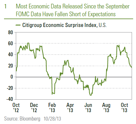
Figure 1 shows the Citigroup Economic Surprise Index for the United States over the past 12 months. The index measures data surprises relative to market expectations. A rising line means that data releases have been stronger than expected, and a falling line means that data releases have been worse than expected. The recent peak in the index came in early September 2013, just prior to the mid-September FOMC meeting. The reports released since mid-September that have fallen short of expectations include:
-
Housing starts (August)
- Richmond Fed Index (September)
- Consumer Confidence (September)
- Durable goods orders and shipments (September)
- Pending home sales (August)
- Markit PMI – Manufacturing (September)
- Vehicle sales (September)
- ISM – Non-Manufacturing (September)
- Small Business Sentiment Index (September)
- Empire State Manufacturing Index (October)
- Existing home sales (September)
- Payroll employment (September)
- Markit PMI – Manufacturing (October)
- Durable goods orders and shipments (October)
How have financial conditions changed since the last FOMC meeting?
The Fed cited tightening financial conditions as one of the reasons it chose not to begin tapering at the September 17 – 18, 2013 FOMC meeting. Figure 2 shows financial conditions – as measured by the Federal Reserve Bank of Chicago’s Financial Conditions Index — have eased since the September FOMC meeting, after tightening over the spring and summer of 2013. Note that despite tightening financial conditions between May and September 2013, they never even got close to where they were during the 2007 – 2009 financial crisis.

Will the FOMC specifically mention the government shutdown in its statement?
There is a strong likelihood that the FOMC statement will mention the recent government shutdown, and the minutes of this week’s FOMC meeting — due out in mid-November 2013 — will almost certainly mention it. The statements released during and just after the 21-day government shutdown in December 1995 and January 1996 did not specifically mention the shutdown, but in those days, FOMC statements were not as verbose as they are today. However, a quick look at the minutes from the December 19, 1995 and January 30 – 31, 1996 meetings finds that both sets of minutes did mention the shutdown and its impact on the economy. The minutes of the January 31, 1996 meeting mentioned the shutdown’s impact on the availability of economic data.
Excerpt from the minutes of the December 19, 1995 FOMC meeting:
The decline in federal purchases in part represented the transitory effects of government shutdowns and the restraining effects of spending cuts imposed by continuing resolutions and by curtailed appropriations in bills that already had been enacted into law.
Excerpts from the minutes of the January 30 – 31, 1996 FOMC meeting:
Only a limited amount of new information was available for this meeting because of delays in government releases…
…these buildups, together with the disruptions from government shutdowns…
The weakness in business activity this winter was to some extent the result of the partial shutdown of the federal government…
What else will we hear from the FOMC this week?
The only communication from the Fed at the conclusion of the meeting will be the FOMC statement, which will be released at 2 PM ET on Wednesday, October 30, 2013. There will be no new economic and interest rate forecast from members of the FOMC, nor will Fed Chairman Ben Bernanke hold a press conference. Market participants will have to wait until the conclusion of the December 17 – 18, 2013 FOMC meeting for the next economic and interest rate forecasts from the FOMC. The press conference following that meeting will be Ben Bernanke’s last as Fed Chairman. We expect that in the near future, the FOMC will strongly consider holding a press conference at each of its eight meetings per year. Many other major central banks across the globe hold press conferences and release forecasts at the conclusion of all of their meetings. In addition, most global central banks hold meetings once a month.
It’s nearly two months away, but what about the next FOMC meeting (December 17 – 18)?
As we noted in last week’s (October 21, 2013) Weekly Economic Commentary: The Lowdown on the Shutdown — The Impact on the Economy and the Fed, the 16-day government shutdown caused delays in the government’s data collection and reporting process for economic data. Since the government’s economic data calendar will not be back to normal until early December, it is unlikely Fed policymakers will announce tapering at the December 17 – 18 FOMC meeting.
An additional hurdle to tapering is the timing of the next government shutdown and debt ceiling debate. Under the terms of the bill passed by Congress in mid-October 2013 to end the shutdown and lift the debt ceiling, the government could shut down again in mid-January 2014, and the Treasury could hit its borrowing limit by early February 2014. While we see this as unlikely, as has been the case in the past few years,these deadlines create uncertainty for the public, market participants, and policymakers and could weigh on economic activity.
In addition, a special bipartisan House-Senate conference committee charged with breaking the impasse on the budget is scheduled to issue a report on December 13, 2013, just days before the December 17 – 18, 2013 FOMC meeting. While a “grand bargain” on the budget might pave the way for the Fed to taper in December 2013, the more likely outcome is that the rancor surrounding this report will only add to the fiscal uncertainty, which argues for a Fed taper in early 2014 and not at the December 17 – 18, 2013 meeting. Of course, if Congress can agree in the next few weeks (for example, by Thanksgiving) on a deal that would eliminate the possibility of another shutdown and bruising debate about the debt ceiling in early 2014, a December taper becomes more likely.
______________________________________________________________________________________________________________________________
IMPORTANT DISCLOSURES
The opinions voiced in this material are for general information only and are not intended to provide specific advice or recommendations for any individual. To determine which investment(s) may be appropriate for you, consult your financial advisor prior to investing. All performance reference is historical and is no guarantee of future results. All indices are unmanaged and cannot be invested into directly.
The economic forecasts set forth in the presentation may not develop as predicted and there can be no guarantee that strategies promoted will be successful.
Stock investing involves risk including loss of principal.
Quantitative easing is a government monetary policy occasionally used to increase the money supply by buying government securities or other securities from the market. Quantitative easing increases the money supply by flooding financial institutions with capital in an effort to promote increased lending and liquidity.
The Federal Open Market Committee (FOMC), a committee within the Federal Reserve System, is charged under the United States law with overseeing the nation’s open market operations (i.e., the Fed’s buying and selling of U.S. Treasury securities).
______________________________________________________________________________________________________________________________
INDEX DESCRIPTIONS
Citigroup Economic Surprise Index (CESI) measures the variation in the gap between the expectations and the real economic data.
The National Financial Conditions Index (NFCI) measures risk, liquidity and leverage in money markets and debt and equity markets as well as in the traditional and “shadow” banking systems. Positive values of the NFCI indicate financial conditions that are tighter than average, while negative values indicate financial conditions that are looser than average.
___________________________________________________________________________________________________________________
This research material has been prepared by LPL Financial.
To the extent you are receiving investment advice from a separately registered independent investment advisor, please note that LPL Financial is not an affiliate of and makes no representation with respect to such entity.
Not FDIC/NCUA Insured | Not Bank/Credit Union Guaranteed | May Lose Value | Not Guaranteed by any Government Agency | Not a Bank/Credit Union Deposit
Member FINRA/SIPC


Trading Partners
September 3, 2013
The upward revision to second quarter gross domestic product (GDP) garnered a great deal of market attention last week (August 26 – 30, 2013). The report, released on Thursday, August 29, revealed that second quarter GDP — initially reported in late July 2013 as a 1.7% gain — was revised higher to a 2.5% gain. All of the upward revision to second quarter GDP can be explained by a narrower trade deficit. Initially, the trade deficit in the second quarter was reported as $451 billion, a 0.8% drag on overall GDP growth. Now, the revised data show that the trade gap stood at “only” 422 billion in the second quarter — the same as in the first quarter of 2013 — and as a result, the economic drag from trade for the quarter was eliminated. Looking ahead to the third quarter of 2013 and beyond, market participants and policymakers are asking: Can trade make a significant positive contribution to GDP growth in the quarters ahead, given the outlook for growth in Europe, China, Japan, and emerging markets?
Tracking the Pace of U.S. GDP Growth
While second quarter GDP was revised higher, the first quarter was not subject to revision and remained at 1.1%, leaving GDP growth in the first half of 2013 at a tepid 1.8%. The Federal Reserve (Fed) is still forecasting a 2.45% gain in GDP this year. With 1.8% growth in real GDP in the first half of the year, real GDP would have to grow by more than 3.0% in the third and fourth quarters of 2013 to match the Fed’s consensus forecast for the year. The Fed will release a revised forecast for the economy, labor markets, and inflation for 2013, 2014, and 2015 on September 18, 2013 at the conclusion of the next Federal Open Market Committee (FOMC) meeting. The FOMC is likely to revise downward its 2013 GDP growth forecast. The new forecast, along with the release of the FOMC’s initial public forecast for the economy, inflation, and the labor market in 2016 (also due on September 18), may help to soothe market fears about the pace of tapering and tightening.
The data in hand for the first two months of the third quarter of 2013 suggest that third quarter GDP is tracking to well under 2%, and may be closer to 1%. The data released thus far for the third quarter of 2013 include:
Data due out this week (September 2 – 6, 2013) on vehicle sales, the Institute for Supply Management (ISM) Purchasing Managers’ Index (PMI), merchandise trade, construction spending, factory shipments and inventories for July and August 2013, and, of course, the August employment report (due out on Friday, September 6) will help to further clarify the pace of GDP growth in the current quarter, the rest of 2013, and into 2014.
GDP Overseas
Data released over the past several months suggest that the economies in Europe and China have stabilized. Meanwhile, market participants have increased their GDP growth forecasts for Japan over the past nine months, as Japanese policymakers have ramped up monetary and fiscal policy and embarked on a series of structural reforms aimed at jarring Japan’s economy out of a multi-decade slumber. Our view remains that while the economies in China and Europe have stopped getting worse, it may take several more quarters before they can meaningfully re-accelerate. While growth has picked up in Japan — second quarter GDP growth in Japan was 2.6% — it remains disappointing relative to elevated expectations. In addition, many emerging market nations (about 50% of U.S. exports head to emerging markets), including India, Brazil, and Indonesia are now experiencing growth and inflation scares, and some (Brazil and Indonesia) are raising interest rates to head off inflation. Many of the market participants and Fed policymakers who expect U.S. GDP to accelerate in the second half of 2013 and in 2014 are likely counting on accelerating growth in Europe, China, Japan, and emerging markets to drive U.S. exports higher. But is that enough to boost U.S. GDP growth?
As noted in our Weekly Economic Commentary: Exporting Good Old American Know-How, from August 19, 2013, the United States has run a trade deficit (importing more goods and services from other countries than it exports) since the mid-1970s, and our large deficit on the goods side (around $759 billion in 2012) more than offsets the trade surplus we have on the service side of the ledger (around $213 billion in 2012). Combined, our goods and services trade deficit was $547 billion in 2012, slightly smaller than the $569 billion deficit in 2011. As a result of the slight narrowing of the deficit between 2011 and 2012, net exports contributed 0.1% to the 2.8% gain in GDP in 2012.
Net Exports Typically Do Not Boost U.S. GDP Growth
The infographic on page 2, “Profile of U.S. Exports” (Profile) reveals that over the past 40 years — aside from recessions (when imports fall faster than exports, narrowing the trade deficit) — net exports have never added more than 1.0% to overall GDP growth. Thus, even if the economies of Europe, China, Japan, and emerging markets accelerate sharply in the next few quarters, it is unlikely that net exports will provide a large boost to GDP growth this year.
In theory, an unexpected uptick in economic activity among our largest export destinations should be a plus for our exports to that region, but in practice, the impact to our trade balance and economy may not immediately reflect the better growth prospects overseas. In addition, exchange rate movements also can influence cross-border trade, but movements often work with a long lag. Since many of our exports do not compete on price, the value of the dollar is not always the best way to gauge the relative strength of our exports to many markets. Generally speaking, U.S. exports compete globally on quality, rather than price.
Export Destinations: Economic Prospects in Canada and Mexico
The Profile details the destinations (trading partners) and mix (goods versus services) of our exports. Fourteen percent of our exports (both goods and services) are bound for the Eurozone, while just 6% head to China. Remarkably, only 5% of our exports go to Japan. Combined, our exports to the Eurozone, Japan, and China account for 25% of our total exports. Closer to home, 16% of our exports head north of the border to Canada, and another 11% head south of the border to Mexico. Thus, our exports to our two closest neighbors (27% of all exports) are larger than our exports to the Eurozone, Japan, and China combined (25%). Accordingly, market participants should probably pay more attention to the economic prospects of Canada and Mexico and a bit less to the prospects of China, the Eurozone, and Japan.
Mix of Goods/Services: Goods Are 70% of All Exports
The Profile also details the goods/services mix of our exports. Currently, goods account for around 70% of all exports, but that varies widely by trading partner. The export mix to Canada and Mexico is skewed toward goods rather than services, which is partially explained by auto production, since auto parts factories and final assembly plants account for such a large portion of trade. Our export mix to the Eurozone, China, and Japan is…well… more mixed. Services, at around 40%, account for more of our trade to the Eurozone and Japan than in our overall trade mix. In China, however, an above-average 78% of our exports are goods. All else being equal, an unexpected and permanent shift higher in economic growth for trading partners like China, the Eurozone, and Japan should boost our exports to those nations over time and, in turn, our GDP. But it is important to note that outside of recessions, net exports rarely add more than 0.5% to GDP growth. So while we spend a great deal of time discussing the health of the economy in China, the Eurozone, Japan, and emerging markets, the economic prospects of our nearest neighbors (Canada and Mexico) have a bigger influence on our overall exports.
______________________________________________________________________________________________________________________________________________________________________________
IMPORTANT DISCLOSURES
The opinions voiced in this material are for general information only and are not intended to provide specific advice or recommendations for any individual. To determine which investment(s) may be appropriate for you, consult your financial advisor prior to investing. All performance reference is historical and is no guarantee of future results. All indices are unmanaged and cannot be invested into directly.
Gross domestic product (GDP) is the monetary value of all the finished goods and services produced within a country’s borders in a specific time period, though GDP is usually calculated on an annual basis. It includes all of private and public consumption, government outlays, investments and exports less imports that occur within a defined territory.
The economic forecasts set forth in the presentation may not develop as predicted and there can be no guarantee that strategies promoted will be successful.
International investing involves special risks, such as currency fluctuation and political instability, and may not be suitable for all investors.
Purchasing Managers Index (PMI) is an indicator of the economic health of the manufacturing sector. The PMI index is based on five major indicators: new orders, inventory levels, production, supplier deliveries and the employment environment.
Markit is a leading, global financial information services company that provides independent data, valuations and trade processing across all asset classes in order to enhance transparency, reduce risk and improve operational efficiency. The Markit Purchasing Managers’ Index (PMIT) is a composite index based on five of the individual indexes with the following weights: New Orders – 0.3, Output – 0.25, Employment – 0.2, Suppliers’ Delivery Times – 0.15, Stocks of Items Purchased – 0.1, with the Delivery Times Index inverted so that it moves in a comparable direction.
The Institute for Supply Management (ISM) index is based on surveys of more than 300 manufacturing firms by the Institute of Supply Management. The ISM Manufacturing Index monitors employment, production inventories, new orders, and supplier deliveries. A composite diffusion index is created that monitors conditions in national manufacturing based on the data from these surveys.
Challenger, Gray & Christmas is the oldest executive outplacement firm in the United States. The firm conducts regular surveys and issues reports on the state of the economy, employment, job-seeking, layoffs, and executive compensation.
This research material has been prepared by LPL Financial.
To the extent you are receiving investment advice from a separately registered independent investment advisor, please note that LPL Financial is not an affiliate of and makes no representation with respect to such entity.
Not FDIC/NCUA Insured | Not Bank/Credit Union Guaranteed | May Lose Value | Not Guaranteed by any Government Agency | Not a Bank/Credit Union Deposit
Member FINRA/SIPC
Posted in Brazil, China, Durable goods, Emerging Markets, Employment, Europe, Eurozone, Exports, Federal Open Market Committee (FOMC), Federal Reserve, GDP - Gross Domestic Product, Goods and Services, India, Institute for Supply Management (ISM), Mexico, Retail Sales, Unemployment, Weekly Economic Commentary | Tagged: Brazil, China, Congress, Durable goods, Emerging markets, employment, Europe, Eurozone, Exports, Fed, federal open market committee, federal reserve, GDP, Goods and Services, India, Institute for Supply Management (ISM), Mexico, Retail Sales, unemployment, Weekly Economic Commentary | Leave a Comment »