Residential Recovery Redux February 25, 2014

Several key reports on the state of the housing market are due out this week (February 24 – 28, 2014), most of which will likely be negatively impacted by the colder and snowier-than-usual weather in much of the nation over December 2013 and January 2014. The data due this week include:

• Case-Shiller Home Price Index for December 2013;
• New Home Sales for January 2014;
• Pending Home Sales for January 2014; and
• Housing Contribution to gross domestic product (GDP) for Q4 2013.

The weather will eventually return to normal, but market participants are likely to be asking: Once the weather improves, will the housing data continue to feel the pinch of higher mortgage rates over the rest of 2014?

Solid Supports

The recent rise in mortgage rates — from just under 3.50% (for a conventional 30-year loan) in May 2013 to a recent reading of just over 4.25% — has led to widespread fears that the housing recovery will come to a grinding halt. Those fears appear to be overdone, in our view, as almost all of the factors supporting an ongoing recovery in housing remain in place. However, the rise in rates will likely slow the pace of the recovery somewhat.

In general, the housing market hit bottom in early 2009, and moved sideways between early 2009 and late 2011 before picking up momentum at the start of 2012 (please see “Location, Location, Location”). Until housing added 0.3 percentage points to overall GDP in 2012, housing construction (the most direct way housing impacts economic growth as measured by GDP) had not been a significant, sustained contributor to economic growth since 2005. The lack of participation from housing has been one of the main reasons for the sluggish economic recovery, along with the severe cutbacks in state and local governments.

When we last wrote in depth on the housing market in mid-2013, we forecast that “despite the recent rapid rise in rates, we still see housing making another significant (0.3 – 0.5 percentage points) contribution to GDP growth in 2013, as the positives driving the residential recovery more than outweigh the negatives.” Indeed, although the data are not final, housing contributed 0.3 percentage points to overall GDP growth in 2013. We expect housing to add between 0.2 and 0.3 percentage points to overall GDP growth in 2014.

At this stage of the recovery, satisfying pent-up demand for housing rather than mortgage rates will likely be the bigger driver of housing. Later on, when the pent-up demand is sated, interest rates (and affordability) should be key drivers, along with housing supply and demand, the willingness of banks and financial institutions to make mortgage loans, the health of the labor market, and the housing PE (median sales price/disposable median income per capita).

Although we continue to hear and read comments from housing market “bears” that the housing market is already back in a “bubble,” housing (represented by residential investment) currently accounts for just 3% of GDP. This is half of what it was at the peak of the housing market in 2005 – 06, when housing accounted for more than 6% of GDP. Since 1980, housing, on average, has accounted for 5% of GDP. At just 3% today, housing’s share of GDP is not only half of the recent peak, but also well below the long-term average of 5%. But what about the other housing indicators?

Key Housing Indicators

Many, if not all, of the other housing indicators we watch (see below) also suggest ongoing recovery in the housing market in the quarters and years to come.

To be sure, while the sharp increase in mortgage rates since mid-May 2013 may have slowed the pace of gains in the U.S. housing market, our view remains that the housing market is still in the early stages of recovering from the 2006 – 09 bust that followed the decade-and-a-half (early 1990s through mid-2000s) housing boom that began to show severe cracks in 2007 and collapsed in 2008. The collapse in housing, in turn, was a major contributor to the financial crisis and the Great Recession of 2007 – 09. The housing market, along with many financial markets and global economies, is still feeling the after-effects of the housing collapse.

The health of the housing market can be measured in many direct ways (e.g., housing starts, housing sales, construction spending, home prices) and indirect ways (e.g., homebuilder sentiment, mortgage applications, foreclosures, inventories of unsold homes, mortgage rates, housing vacancies, lumber prices, prices of publicly traded homebuilders). The U.S. government and private sources collect and disseminate these data. A quick recap of some of these indicators is below.

Taking the Pulse of the Residential Recovery

• Near-record housing affordability. Housing affordability, the ability of a household with the median income to afford the payments on a median priced house at prevailing mortgage rates, hit an all-time high in early 2013 before the big run-up in mortgage rates that began in mid-May 2013. The latest data point (December 2013) saw a 21% drop in affordability from the peak in January 2013. Despite the drop, affordability remains well above the long-term average, and it is some 70% higher than at the peak of the housing market in late 2005/early 2006. Rising incomes and the aftermath of the 20 – 30% drop in home prices nationwide between 2005 and 2009 will continue to support an elevated level of affordability. At this point in the housing recovery, pent-up demand will likely outweigh affordability as the main driver of housing demand.
• The housing PE. Although not a perfect measure of the frothiness (or lack thereof) in the housing market, the ratio of the median sales price of an existing home ($197,700 in December 2013) to disposable personal income per capita ($39,726 as of December 2013) is one way to gauge the health of the market. Our infographic shows that while the housing PE”has moved higher in recent months, it remains well below average. Indeed, aside from the housing bust era (2007 – 11), the housing PE is the lowest it has been in more than four decades. This also suggests that the housing recovery remains in its early stages and is not in a bubble.
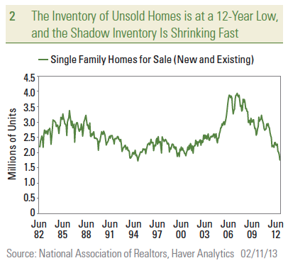
• Inventories of unsold homes are tight. Although the inventory of unsold new and existing homes has moved up from a 32-year low since the start of 2013, inventories of unsold homes remain well below average. The official count of the inventory of unsold single-family existing homes (from the National Association of Realtors), along with the record-low inventory of new homes for sale, tells us 1.8 million homes are for sale. Depending on the data source cited (there is no “official” number for shadow inventory), the shadow inventory is in the 1.0 – 1.5 million range. The low inventory of unsold homes, particularly in areas where housing demand is the highest, supports ongoing improvement in housing construction and housing sales.
• Supply of home mortgages. From the mid-1990s through late 2006, bank lending standards (down payment required, credit scores, work history, etc.) for residential mortgages were relatively easy. Coupled with low rates and rapid innovation in financial products backing residential mortgages, this easy credit helped to fuel the housing boom. The banking industry began tightening lending standards in early 2007, and continued to tighten for more than two years. Lending standards eased in 2009 and 2010, but remained more restrictive than they were in the peak boom years from 2004 to 2006. The latest survey (February 2014) reveals that bank lending standards for home mortgages are now back to “normal,” as defined by the 10 years between 1995 and 2005. It’s too soon to tell whether or not the tightening of standards in the latest period (February 2014) is the start of a new trend, or just a wiggle in the data. Either way, relatively normal mortgage lending standards are supportive of more gains in housing in the coming quarters. The Federal Reserve (Fed) compiles these data in the quarterly Senior Loan Officer Survey.
• Demand for home mortgages. Consumer demand for mortgages remained muted during the first two-and-a-half years (early 2009 through late 2011) of the housing recovery, as consumers remained uncertain about prospects for home price appreciation and their own financial and labor market status. Between mid-2011 and mid-2013, an improving labor market, Fed actions to lower mortgage rates, and rising home prices drove consumer demand for mortgages to levels not seen since the early 2000s. But the rise in mortgage rates since mid-2013 has had a meaningful impact on demand for mortgage loans in recent quarters, and a further pullback in consumer demand for mortgages would be a threat to the sustainability of the recovery. The housing recovery is dependent upon low interest rates, but not necessarily the lowest interest rates. History shows us that if job and income growth can rise along with mortgage rates, the growth in housing can continue. The Fed compiles these data in the quarterly Senior Loan Officer Survey.
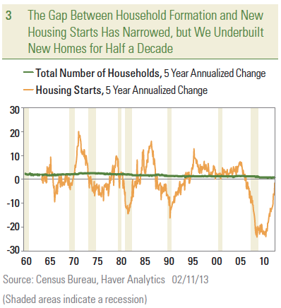
• Demand for housing. Net household formation boomed in the mid- 2000s (2004, 2005, and 2006) but began to slow just prior to the start of the Great Recession in 2007. Unemployed new graduates were living with their parents or renting in large groups rather than moving into homes of their own for years after the 2007 – 09 recession. But that is ending. Over the past five years, (2009 – 13) household formations have stabilized, partially due to the better labor market, but also thanks to the echo boomers reaching their mid-to-late 20s. Although new household formation has slowed from its pre-Great Recession pace, it is still running at almost 1.0% per year. By early 2011, the gap between new household formation and new housing starts had never been wider. Soon thereafter, housing starts began to recover, and the healing in the housing market began to accelerate. However, there are still more than 18 million vacant homes — down from the peak of more than 19 million, but still well above the pre-Great Recession level of 14 – 15 million. This indicator continues to suggest that the housing recovery is still in its early stages. The U.S. Census Bureau collects the data on household formation and housing vacancies.

On balance, the sharp rise in mortgage rates that commenced in mid- May 2013 will likely slow the pace of housing activity that had accelerated noticeably between mid-2011 and mid-2013. Despite the rise in rates, most of the indicators we watch suggest that the housing recovery remains firmly entrenched. The pace (and sustainability) of the housing recovery will help to determine the pace of the overall economic recovery. We expect housing — as measured by the residential investment component of GDP — to make a positive contribution to overall GDP growth in 2014, as it did in both 2012 and 2013. However, it will likely take several more years before the national housing market is back to normal.

______________________________________________________________________________________________________________________________

IMPORTANT DISCLOSURES

The opinions voiced in this material are for general information only and are not intended to provide specific advice or recommendations for any individual. To determine which investment(s) may be appropriate for you, consult your financial advisor prior to investing. All performance reference is historical and is no guarantee of future results. All indices are unmanaged and cannot be invested into directly.

The economic forecasts set forth in the presentation may not develop as predicted and there can be no guarantee that strategies promoted will be successful.

Gross Domestic Product (GDP) is the monetary value of all the finished goods and services produced within a country’s borders in a specific time period, though GDP is usually calculated on an annual basis. It includes all of private and public consumption, government outlays, investments and exports less imports that occur within a defined territory.

______________________________________________________________________________________________________________________________

This research material has been prepared by LPL Financial.

To the extent you are receiving investment advice from a separately registered independent investment advisor, please note that LPL Financial is not an affiliate of and makes no representation with respect to such entity.

Not FDIC/NCUA Insured | Not Bank/Credit Union Guaranteed | May Lose Value | Not Guaranteed by any Government Agency | Not a Bank/Credit Union Deposit

Member FINRA/SIPC

Guide to Q1: Global Growth, Jobs, and the Fed January 7, 2014

LPL Financial Research forecasts U.S. economic growth, as measured by real gross domestic product (GDP), to accelerate to 3% in 2014 from the 2% pace of recent years. This marks our first above-consensus annual forecast for GDP in many years. As of mid-December 2013, the Bloomberg-tracked consensus estimate by economists for 2014 was 2.6%. If achieved, the 3% pace of GDP growth in 2014 would be the best performance for the U.S. economy since 2005, when the economy posted 3.4% growth. While a strong growth rate in comparison to the past 10 years, the 3% growth rate would simply equal the average pace of real GDP growth since the end of WWII.

Global GDP growth is also likely to accelerate in 2014. The economists’ consensus forecast expects a pickup from around 3% in 2013 to 3.5% in 2014. Beyond the United States, the major contributors to this growth rate amay also enjoy a better pace of growth in 2014:

• Europe will likely eke out a modest gain in GDP after emerging from a double-dip recession in 2013;
• China’s growth should stabilize in the coming year after slowing during the last few years; and
• Japan could record its third consecutive year of GDP growth for the first time since the mid-2000s.

Below, we take a month-by-month look at what could be some of the key milestones for the economic outlook in the first quarter of 2014.

January:

• 19th: China’s GDP report for 2013 – As of mid-December 2013, the consensus of economists polled by Bloomberg News expected that China’s GDP growth in 2013 would be between 7.5% and 8.0%, close to the 7.7% gain in 2012, but far below the 10 – 12% pace set by the Chinese economy between 2000 and 2007. In our view, markets have yet to become comfortable with the notion that China may never again see 10% GDP growth on a sustained basis, as it continues its transition from an export-led economy to a more stable, consumer-led economy. 
• 29th: First of eight Federal Open Market Committee (FOMC) meetings for 2014 – The Federal Reserve (Fed) is expected to maintain the current pace of tapering ($10 billion less in purchases) of quantitative easing at this meeting. The pace of the economy in 2014 will determine how quickly the Fed trims its purchases.

This is Janet Yellen’s first meeting as Chairwoman of the Fed and FOMC, the policymaking arm of the Fed. We continue to expect that Yellen will aim for more transparency at the Fed in 2014, and that could mean a press conference after each of the eight FOMC meetings this year. Currently, Yellen is scheduled to hold only four press conferences—after the March, June, September, and December 2014 FOMC meetings.

• 30th: The first estimate of GDP for Q4 2013 will be released – The government shutdown in the first half of October 2013 likely weighed on growth and based on the daily, weekly, and monthly data already in hand for the fourth quarter of 2013, fourth quarter 2013 GDP is currently tracking to around 2.0%. If GDP does come in at around 2.0% in the fourth quarter, GDP growth for all of 2013 would be just 1.9%.

February:

• 7th: Employment report for January 2014 will be released – The pace of job growth is one of the keys to the pace of Fed tapering in 2014. The December 2013 jobs report (due out this Friday, January 10, 2014) will likely show that the economy again created a net new 200,000 jobs in December 2013, close to the pace of job creation seen over the past three, six, and 12 months. If job creation increases markedly from this pace, the market will expect the Fed to quicken its pace of tapering. Similarly, a sustained slowdown in job creation from the current 200,000 per-month pace might cause the Fed to slow its tapering plan.

• 14th: Eurozone will report GDP for Q4 2013 and all of 2013 – The Eurozone is expected to have eked out a modest (0.4%) increase in GDP in the fourth quarter of 2013, which would leave GDP for all of 2013 0.4% below its 2012 level. Looking ahead to 2014, the Bloomberg consensus estimate for Eurozone GDP (as of mid-December 2013) stands at just 1.0%, still among the slowest growth in the developed world. While the European economy stopped getting worse in 2013, it is not likely to improve dramatically until it can effectively address its broken financial transmission mechanism. The latest data show that while money supply growth in the Eurozone is slightly positive, bank lending to small and medium-sized businesses in the Eurozone is still contracting — and at a faster rate than it was at the start of 2013 [Figure 1]. We view this as a key impediment to faster economic growth in the Eurozone in 2014.

• Late February: Retailers will report their sales and earnings for their fiscal fourth quarters, the three months ending in January 2014. – These results will serve as the final say on the 2013 holiday shopping season. The improvement in the labor and housing markets throughout 2013, as well as the increases in household net worth, driven in part by the 25 – 30% gain in equity prices in 2013 to new all-time highs, will act as support for holiday spending. Most retailers will report their December 2013 sales and provide guidance for January 2014 and beyond later this week (Thursday, January 9, 2014).

March

• 4th: Q4 2013 Flow of Funds report will be released by the Fed – The quarterly flow of funds report is often ignored by markets and the media, as it is difficult to interpret and is released with a long lag. However, the report is full of crucial data, including household balance sheets (assets and liabilities). The latest data available (Q3 2013) revealed that household net worth (assets minus liabilities) hit another new all-time high in the third quarter [Figure 2], aided by solid gains in the labor market, home prices, and sizable increases in financial assets, like equities. All of those categories continued to move higher in the fourth quarter of 2013, suggesting that household net worth will likely hit another all-time high in the fourth quarter of 2013. The rise in household net worth provides solid support for consumer spending, which represents two-thirds of GDP.

• 19th: FOMC meeting – If the Fed sticks to its current communications plan, March 19, 2014 will be Janet Yellen’s first press conference as Fed Chairwoman. As noted above, we expect Yellen to continue to enhance the Fed’s transparency over the course of 2014.

• 31st: Start of the 58th month of the economic expansion that began in July 2009 – As noted in our Outlook 2014 publication, since the end of WWII, the average economic expansion has lasted 58 months [Figure 3]. Looking back over the past 50 years, the average expansion has been 71 months. On that basis, the current recovery has another two years to go (2014 and 2015) just to get to “average.” The best comparison, however, may be the three economic expansions since the end of the inflationary 1970s, a period that has seen the transformation of the U.S. economy from a domestically focused, manufacturing economy to a more exportheavy, service-based economy. In general, this economic structure is less prone to inventory swings that drove the shorter boom-bust cycles of the past. On average, the last three expansions — the ones that began in 1982, 1991, and 2001 — lasted 95 months, or roughly eight years. Using those three expansions as the standard, the current economic expansion would merely be at its midpoint at the end of March 2014. The rather tepid pace of this expansion relative to prior expansions that lasted this long also supports the idea that we are close to the middle of the expansion, rather than the end.

_____________________________________________________________________________________________________________________________

IMPORTANT DISCLOSURES

The opinions voiced in this material are for general information only and are not intended to provide specific advice or recommendations for any individual. To determine which  investment(s) may be appropriate for you, consult your financial advisor prior to investing. All performance reference is historical and is no guarantee of future results. All indices are unmanaged and cannot be invested into directly.

The economic forecasts set forth in the presentation may not develop as predicted and there can be no guarantee that strategies promoted will be successful.

Stock investing involves risk including loss of principal.

The Federal Open Market Committee (FOMC), a committee within the Federal Reserve System, is charged under the United States law with overseeing the nation’s open market operations (i.e., the Fed’s buying and selling of U.S. Treasury securities).

Quantitative easing is a government monetary policy occasionally used to increase the money supply by buying government securities or other securities from the market. Quantitative easing increases the money supply by flooding financial institutions with capital in an effort to promote increased lending and liquidity.

Tapering refers to the Federal Reserve (Fed) slowing the pace of bond purchases in their Quantitative Easing (QE) program. To execute QE, the Fed purchases a set amount of Treasury and Mortgage-Backed bonds each month from banks. This inserts more money in the economy (known as easing), which is intended to encourage economic growth. Lowering the amount of purchases (tapering) would indicate less easing of monetary policy.

_____________________________________________________________________________________________________________________________

This research material has been prepared by LPL Financial.

To the extent you are receiving investment advice from a separately registered independent investment advisor, please note that LPL Financial is not an affiliate of and makes no representation with respect to such entity.

Not FDIC/NCUA Insured | Not Bank/Credit Union Guaranteed | May Lose Value | Not Guaranteed by any Government Agency | Not a Bank/Credit Union Deposit

Member FINRA/SIPC

Measuring Economic Expansion August 13, 2013

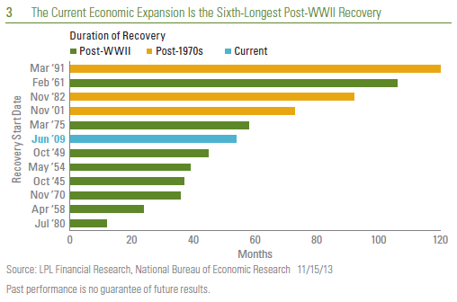
The U.S. economy is now in the fifth year of the 12th economic recovery (or expansion) since the end of World  War II. It is already the sixth-longest expansion and would have to last another year to become the fifth longest, as discussed in last week’s Weekly Economic Commentary: Revisiting the Recovery. This week, we will  compare the performance of gross domestic product (GDP) — the broadest measure of economic activity —  and its components (consumer spending, business capital spending, government spending, etc.) in the current  recovery to previous economic recoveries.

Where We Stand vs. Prior Recoveries

The Great Recession of 2007 – 2009 ended in the second quarter of 2009, and the economy has been growing  for 16 quarters now. Of the other 11 economic expansions since the end of WWII, just five lasted at least four years — the recoveries that began in 1961, 1975, 1982, 1991, and 2001. By the end of their fourth year in the five  expansions that lasted 16 quarters or more (or “comparable recoveries”), real GDP, on average, had  increased by a cumulative 19% from the end of (or trough) the prior recession. In the current expansion, the  economy has grown by just 9% over the last four years (from $14.4 trillion in Q209 to $15.6 trillion in Q213) [Figure 1].

The Pace of GDP

Consumer spending, which accounts for more than two-thirds of GDP, has matched the performance of overall GDP in this expansion, growing 9% from the trough versus an average 18% gain from the trough in the other five post WWII comparable recoveries. With the exception of exports, all the other major components of GDP — business capital spending, housing, business spending on structures (office parks, malls, factories, etc.),  exports and government spending — have badly underperformed the average post-WWII recovery. Why has  the current recovery been so lackluster even after such a severe recession?

Several factors along with uncertainty over legislative and regulatory policy in Washington have contributed to weak growth, not only in consumption, but in all the sectors of the economy over the past four years. These factors include strained balance sheets, only modest gains in the labor market, banks’ unwillingness to lend after billions of losses in the housing bust, and a weak external environment (recession in Europe, slowdown in China, and emerging markets).

While the current expansion has lagged comparable expansions in almost every category of GDP, it may not be an “apples-to-apples” comparison. As we noted in last week’s Weekly Economic Commentary, the U.S. economy has changed significantly since the end of the inflationary 1970s. The last 30-plus years has seen the  transformation of the U.S. economy from a domestically focused manufacturing economy to a more export- heavy, service-based economy. In general, this economic structure is less prone to inventory swings that drove  the shorter boom-bust cycles of the past, and has led to longer expansions. On average, the last three expansions — the ones that began in 1982, 1991, and 2001 — lasted 95 months, or roughly eight years. Using those three expansions as the standard, at 49 months (16 quarters) the current economic expansion is at its midpoint, but it has been far less robust.

Using just the last three economic expansions for comparison, the pace of GDP growth in the past four years  still lags the average. GDP grew by 16% over the first four years of the last three expansions, and even by that standard the current recovery (9%) is not up to par. Still, in every major category — except exports, where the current recovery matches the prior three — the current expansion falls short, in some cases far short, of the past three recoveries, especially in government spending, housing, and business investment in structures. Taking the Pulse of Government Spending Government spending in all post-WWII expansions has generally not kept pace with overall growth in GDP. Four years into the average post-WWII expansion, government spending (federal, state, and local) has increased, by 10%, about half of the increase in overall GDP (20%) [Figure2]. In the past 30 years, government spending in the first four years of expansion has increased, on average, by just 9%, lagging the overall pace of economic activity but still adding to growth. However, in the current expansion, government spending has decreased by 6%, with state and local government spending taking the biggest hit (down 8% from the second quarter of 2009). At the federal level, overall spending is down 5% from the second quarter of 2009, with an 8% cut to defense spending more than offsetting a 4% increase in non-defense  spending.

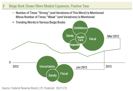
Spending at the state and local level is now stabilizing, after more than five years of spending cuts. At the  federal level, the impact of the sequester, the fiscal cliff, and defense cuts were still reverberating through the economy as the second half of 2013 began. On balance, government spending should be less of a drag on growth in the next four years than it was in the first four of the recovery, when government spending added to growth in only three of 16 quarters.

Taking the Pulse of the Housing Market

Although it got a late start, housing — at the epicenter of the Great Recession — has outperformed the overall  economy over the past four years (as it typically does during expansions), but underperformed relative to its performance in past expansions. Housing (as measured by investment in new residential structures) has increased by 30% over the past four years, far above the 9% gain in GDP in that span. But the 30% gain pales in comparison to the 50% average gain in housing in the first four years of all post-WWII recoveries, and also falls  far short of the 51% average gain in housing during the past three expansions (1982, 1991, and 2001). The hangover from the housing bust (large amounts of unsold inventory, difficulty in obtaining financing, poor consumer credit profiles, and a lackluster labor market) helps explain housing’s underwhelming performance in this recovery.

Looking ahead, our view remains that housing is in the early stages of a long recovery, aided by pent-up  demand, near record-low inventories, near record-high housing affordability, a steadily improving labor market, and banks’ increased willingness to lend to borrowers. The recent rise in mortgage rates is a concern, but will likely only slow, not stop, the ongoing recovery in housing, which is being driven, in part, by cash buyers and pent-up demand.

Taking the Pulse of Business Investment in New Structures

On average, business investment in new structures (shopping malls, office buildings and office parks, factories, etc.) over the first four years of all post-WWII expansions rose 6%, lagging the pace of the average recovery in GDP (19%) [Figure 2]. Why does business investment in structures lag overall growth? In part, because these are typically very large projects with long lead times and require outsized commitments of capital, so  businesses want to make sure the expansion is well entrenched before committing resources. As a result, this segment of GDP tends to lag during the early part of expansions and then picks up steam as the expansion matures. We would expect the same pattern to repeat in the current expansion.

In the three expansions since 1980, business investment on structures actually dropped by 7% over the first 16  quarters of the expansion, lagging the average of all post-WWII expansions (a 6% gain over four years). But the current expansion has seen business investment in structures fall by 9% over the past four years, an even worse performance than in the past three expansions (a 7% decrease). Business uncertainty around the health and longevity of the expansion, the turmoil in Europe and slowdown in China, as well as the legislative and regulatory backdrop, overwhelmed the positive impact of lower financing rates and years of pent-up demand. We expect business investment in structures to pick up steam and become a bigger contributor to growth in  the second half of the expansion, aided by somewhat less legislative and regulatory concern and more confidence in the economy.

Taking the Pulse of Business Investment in New Structures

On average, business investment in new structures (shopping malls, office buildings and office parks, factories, etc.) over the first four years of all post-WWII expansions rose 6%, lagging the pace of the average recovery in GDP (19%) [Figure 2]. Why does business investment in structures lag overall growth? In part, because these  are typically very large projects with long lead times and require outsized commitments of capital, so businesses want to make sure the expansion is well entrenched before committing resources. As a result, this segment of GDP tends to lag during the early part of expansions and then picks up steam as the expansion matures. We would expect the same pattern to repeat in the current expansion.

In the three expansions since 1980, business investment on structures actually dropped by 7% over the first 16 quarters of the expansion, lagging the average of all post-WWII expansions (a 6% gain over four years). But the current expansion has seen business investment in structures fall by 9% over the past four years, an even worse performance than in  the past three expansions (a 7% decrease). Business uncertainty around the health and longevity of the expansion, the turmoil in Europe and slowdown in China, as well as the legislative and regulatory backdrop,  overwhelmed the positive impact of lower financing rates and years of pent-up demand. We expect business  investment in structures to pick up steam and become a bigger contributor to growth in the second half of the  expansion, aided by somewhat less legislative and regulatory concern and more confidence in the economy.

Expansion Lagging Average Post-WWII Recovery

Although it is four years old, the current economic expansion has not felt like a real expansion to many consumers and businesses. Indeed, the data suggest that in virtually every segment of the economy, the current expansion has lagged the average post-WWII expansion and the three expansions since 1980, which are more comparable. While some of the factors that have weighed on the expansion are lifting, others, notably rising interest rates, are poised to take their place and we continue to expect modest (near 2.0%) growth in 2013.

______________________________________________________________________________________________________________

IMPORTANT DISCLOSURES

The opinions voiced in this material are for general information only and are not intended to provide specific advice or recommendations for any individual. To determine which investment(s) may be appropriate for you, consult your financial advisor prior to investing. All performance reference is historical and is no guarantee of future results. All indices are unmanaged and cannot be invested into directly.

The economic forecasts set forth in the presentation may not develop as predicted and there can be no guarantee that strategies promoted will be successful.

Gross domestic product (GDP) is the monetary value of all the finished goods and services produced within a country’s borders in a specific time period, though GDP is usually  calculated on an annual basis. It includes all of private and public consumption, government outlays, investments and exports less imports that occur within a defined territory.

The Federal Open Market Committee (FOMC), a committee within the Federal Reserve System, is charged under the United States law with overseeing the nation’s open market operations (i.e., the Fed’s buying and selling of United States Treasure securities).

Quantitative easing is a government monetary policy occasionally used to increase the money supply by buying government securities or other securities from the market.  Quantitative easing increases the money supply by flooding financial institutions with capital in an effort to promote increased lending and liquidity.

This research material has been prepared by LPL Financial.

To the extent you are receiving investment advice from a separately registered independent investment advisor, please note that LPL Financial is not an affiliate of and makes no representation with respect to such entity

Not FDIC/NCUA Insured | Not Bank/Credit Union Guaranteed | May Lose Value | Not Guaranteed by any Government Agency | Not a Bank/Credit Union Deposit

Member FINRA/SIPC

Listening to the leaders May 14, 2013

Leading Indicators Continue to Point to Slow Economic Growth, but no Recession

The April Index of Leading Economic Indicators (LEI), due out on Friday, May 17, 2013, caps off a busy week for economic reports in the United States. This week includes reports on:

• The consumer: Retail sales for April 2013 and the University of MichiganIndex of Consumer Sentiment for early May 2013;
• Housing: Housing starts and building permits for April 2013 and the National Association of Homebuilders sentiment index for May 2013;
• Manufacturing: Empire State Manufacturing Index for May, the Philadelphia Fed Manufacturing Index for May 2013, industrial production and capacity utilization for April 2013; and
• Inflation: Consumer Price Index (CPI) and Producer Price Index (PPI) for April 2013.

On balance, these reports are likely to continue to show that the U.S. economy is growing at around 2.0% in the second quarter of 2013, that inflation remains muted, and that the odds of a recession in the next year to 18 months remains low. Policymakers at the Federal Reserve (Fed) will digest all of this data, and likely conclude that its quantitative easing (QE) program — the purchase of $85 billion per month of Treasury securities — should continue over the remainder of 2013.

LEI Updates

If you have not seen the LEI lately, there have been several changes made to its components, although as before, virtually all of the components of the LEI are known before the data are actually released. So in theory, the LEI itself should not be a surprise to market participants, the media, or pundits. Of course, that will not prevent anyone from ascribing movements in financial markets on Friday, May 17 to the LEI data, but we are always quick to point out that the S&P 500 itself is a component in the LEI.

In December 2011, the Conference Board, the private “think tank” that compiles and releases the data each month, made four changes to the LEI:

• The Conference Board’s proprietary “Leading Credit Index” (LCI), an aggregate of several well-known financial market and credit market metrics like swap spreads, investor sentiment, margin account, etc., replaced the inflation adjusted M2 money supply.
• The Institute for Supply Management’s (ISM) New Orders Index replaced the ISM’s Supplier Deliveries Index.
• The U.S. Department of Census’ new orders for non-defense capital goods excluding aircraft replaced new orders for non-defense capital goods.
• A combination of consumer expectations and business and economic conditions replace the University of Michigan’s Consumer Expectations Index.

LEI Places Very Low Odds of Recession in Next 12 Months

According to the consensus estimates compiled by Bloomberg News, the LEI is expected to post a 0.2% month-over-month gain in April 2013. The expected 0.2% month-over-month gain would put the year-over-year gain in the LEI at 2.1%. The LEI is designed to predict the future path of the economy, with a lead time of between six and 12 months. Since 1960 — 640 months or 53 years and four months — the year-over-year increase in the LEI has been at least 2.1% in 397 months. Not surprisingly, the U.S. economy was not in recession in any of those 397 months. Thus, it is highly unlikely that the economy was in recession in April 2013, despite the impact of the sequester, the fiscal cliff (spending cuts, payroll tax increases, income tax rate increases, etc.), the recession in Europe, or the slowdown in China.

But the LEI is designed to tell market participants what is likely to happen to the U.S. economy, not what has already happened. Three months after each of the 397 months that the LEI was up 2.1% or more, the economy was in recession in just two of the 397 months — both in 1973. Six months after the LEI was up by 2.1% or more on a year-over-year basis, the U.S. economy has been in recession in just six of the 397 months or 2% of the time. Looking out 12 months after the LEI was up 2.1% or more, the economy was in recession in just 27 of the 397 months, or 7% of the time. Based on this relationship, the odds of a recession within the next 18 months and two years increase to between 10% and 15%.

On balance, the LEI says the risk of recession in the next 12 months is negligible (7%), but not zero. We would agree. But, the still-fragile state of the economy, and the uncertainty surrounding domestic fiscal policy, the recession in Europe, and the ongoing slowdown in China are telling us that the risk of recession is much higher than 7%. Our view remains that — aided by the Fed’s QE program, the early stages of a housing recovery, and a nascent manufacturing recovery — the U.S. economy is likely to grow at around 2.0% this year. The full impact of the sequester, the looming debate over the federal debt ceiling, weak exports, and ongoing contraction in both federal and state and local government spending are all acting to restrain growth, and these factors are likely to be in place for most of this year. A dramatic deterioration of the fiscal and financial situation in Europe, a fiscal or monetary policy mistake here in the United States or abroad, or an exogenous event (a major terror attack, natural disaster, etc.), among other events, may cause us to change our view.

______________________________________________________________________________________________________________________________________________

IMPORTANT DISCLOSURES
The opinions voiced in this material are for general information only and are not intended to provide specific advice or recommendations for any individual. To determine which investment(s) may be appropriate for you, consult your financial advisor prior to investing. All performance reference is historical and is no guarantee of future results. All indices are unmanaged and cannot be invested into directly.

* Over the last three quarters (third quarter of 2012, fourth quarter of 2012, and first quarter of 2013) , real GDP growth has averaged 2.0%.

Gross domestic product (GDP) is the monetary value of all the finished goods and services produced within a country’s borders in a specific time period, though GDP is usually calculated on an annual basis. It includes all of private and public consumption, government outlays, investments and exports less imports that occur within a defined territory.

The economic forecasts set forth in the presentation may not develop as predicted and there can be no guarantee that strategies promoted will be successful.

Stock investing involves risk including loss of principal.

Quantitative easing is a government monetary policy occasionally used to increase the money supply by buying government securities or other securities from the market. Quantitative easing increases the money supply by flooding financial institutions with capital in an effort to promote increased lending and liquidity.

The Federal Open Market Committee (FOMC) , a committee within the Federal Reserve System, is charged under the United States law with overseeing the nation’s open market operations (i.e., the Fed’s buying and selling of U.S. Treasury securities).

The Congressional Budget Office is a non-partisan arm of Congress, established in 1974, to provide Congress with non-partisan scoring of budget proposals.

______________________________________________________________________________________________________________________________________________

INDEX DESCRIPTIONS
The Consumer Price Index (CPI) is a measure of the average change over time in the prices paid by urban consumers for a market basket of consumer goods and services.

The Empire State Manufacturing Index is a seasonally-adjusted index that tracks the results of the Empire State Manufacturing Survey. The survey is distributed to roughly 175 manufacturing executives and asks questions intended to gauge both the current sentiment of the executives and their six-month outlook on the sector.

The Institute for Supply Management (ISM) index is based on surveys of more than 300 manufacturing firms by the Institute of Supply Management. The ISM Manufacturing Index monitors employment, production inventories, new orders, and supplier deliveries. A composite diffusion index is created that monitors conditions in national manufacturing based on the data from these surveys.

The index of leading economic indicators (LEI) is an economic variable, such as private-sector wages, that tends to show the direction of future economic activity.

The Leading Credit Index constitutes financial market indicators including bond market yield curve data, interest rate swaps, and Fed bank lending survey data.

The NAHB/Wells Fargo Housing Market Index gauges builder perceptions of current single-family home sales and sales expectations for the next six months as “good,” “fair” or “poor.” The survey also asks builders to rate traffic of prospective buyers as “high to very high,” “average,” or “low to very low.” Scores from each component are then used to calculate a seasonally adjusted index where any number over 50 indicates that more builders view conditions as good than poor.

The Philadelphia Fed Manufacturing Index is a survey produced by the Federal Reserve Bank of Philadelphia, which questions manufacturers on general business conditions. The index covers the Philadelphia, New Jersey, and Delaware region. Higher survey figures suggest higher production, which contribute to economic growth. Results are calculated as the difference between percentage scores with zero acting as the centerline point. As such, values greater than zero indicate growth, while values less than zero indicate contraction.

The Producer Price Index (PPI) program measures the average change over time in the selling prices received by domestic producers for their output. The prices included in the PPI are from the first commercial transaction for many products and some services.

Purchasing Managers’ Index (PMI) is an indicator of the economic health of the manufacturing sector. The PMI index is based on five major indicators: new orders, inventory levels, production, supplier deliveries, and the employment environment.

The University of Michigan Consumer Sentiment Index (MCSI) is a survey of consumer confidence conducted by the University of Michigan. The Michigan Consumer Sentiment Index (MCSI) uses telephone surveys to gather information on consumer expectations regarding the overall economy.

______________________________________________________________________________________________________________________________________________

This research material has been prepared by LPL Financial.
To the extent you are receiving investment advice from a separately registered independent investment advisor, please note that LPL Financial is
not an affiliate of and makes no representation with respect to such entity.

Not FDIC/NCUA Insured | Not Bank/Credit Union Guaranteed | May Lose Value | Not Guaranteed by any Government Agency | Not a Bank/Credit Union Deposit

The ABC’s of GDP April 30, 2013

The ABC’s of GDP

GDP = C + I + G + (X-M)

College freshmen know it — or should know it — by the end of their Economics 101 classes, but for most of us, freshman year in college remains a bit “fuzzy” for a variety of reasons. On Friday, April 26, 2013, the Bureau of Economic Analysis (BEA) of the U.S. Department of Commerce released the first estimate of gross domestic product (GDP) for the first quarter of 2013. Inflation-adjusted, or real, GDP expanded at a 2.5% seasonally adjusted annualized rate in the first quarter of 2013, after rising at just 0.4% in the fourth quarter of 2012. The 2.5% increase fell short of expectations for 3.0% growth. Over the last three quarters (third quarter of 2012, fourth quarter of 2012, and first quarter of 2013), real GDP growth has averaged 2.0%. We continue to expect GDP growth to average around 2.0% over the course of 2013.

Although consumer spending, housing, and inventory accumulation accelerated in Q113 versus Q412 and added to growth, business spending slowed dramatically, and the trade deficit widened, dampening growth.  Housing construction added 0.3 percentage points to GDP in the first quarter, marking the eighth quarter in a row that housing has added to GDP, after a five-year period (2006 – 2010) where housing was a drag on GDP.

The big story in the GDP report was again federal government spending.  Defense spending fell 11.5% annualized between Q412 and Q113, after the 22% drop in Q412 versus Q312, the largest back-to-back drop in defense spending in 60 years. The sequester, which cut federal government spending across the board beginning on March 1, 2013, contributed to a 2.0% drop in non-defense federal spending between Q412 and Q113. State and local government spending fell again, too, by 1.2% between Q413 and Q113, the second consecutive quarterly decline, and the 13th quarterly decline in state and local spending in the past 14 quarters, dating back to the end of 2009. On balance, there were few, if any signs, in the GDP report for the first quarter of 2013 that the economy will re-accelerate anytime soon.

The ABC’s of GDP
 A – (Seasonally) adjusted. GDP is reported by the BEA in several different ways, but the most commonly cited way is on a real (inflation-adjusted) seasonally adjusted annualized basis. GDP is seasonally adjusted to smooth out the fluctuation in the economy related to weather patterns, shopping patterns, holidays, school vacations, etc., to allow apples-to-apples comparisons between quarters. For example, vehicle assembly plants typically shut down in July, which would depress GDP in the third quarter (July, August, and September) relative to the second quarter (April, May, and June). Similarly, sales of jewelry spikes around Christmas and again at Valentine’s Day. Seasonally adjusting the data helps market participants to see through the swings in the seasonal data and helps to reveal the true underlying health of the economy at any time of the year.

B – Business capital spending. Part of “I,” business capital spending (capex), is what businesses spend on machinery, software, furniture, vehicles, computers, iPads, etc.  Businesses spent an annualized $1.2 trillion on equipment and software in the first quarter of 2013, accounting for 8% of GDP.  Business capital spending is very sensitive to economic conditions.  Business capital spending did not surpass its pre-Great Recession peak of $1.1 trillion until mid-2012. Market participants digest plenty of “input” data on business capital spending — Institute for Supply Management (ISM), durable goods orders and shipments, the regional Federal Reserve Bank manufacturing indices, reports from companies, truck sales, steel production, and rail car loadings — well ahead of the GDP report, but there is more information available to gauge consumer spending than there is to gauge business spending.

C – Consumption or consumer spending, on durable goods, non-durable goods, and services.  Consumption accounts for two-thirds of GDP. In the first quarter of 2013, consumers spent an annualized $9.7 trillion, adjusted for inflation. Consumption surpassed its pre-Great Recession peak of $9.3 trillion in early 2011. Of all the categories of GDP, consumption is the most visible to most consumers. We all spend money on various items every day. The data sets that provide input to the consumption portion of GDP — weekly retail sales, chain store sales, vehicle sales, etc. — is both robust and abundant. By the time GDP is released, most market participants have a pretty good sense of what this component of GDP is doing.

D – Durable goods. Consumer spending on durable goods (items designed to last more than three years), including microwave ovens, refrigerators, and color TVs. Consumers spent an annualized $1.4 trillion on durable goods in the first quarter of 2013. Spending on durable goods surpassed the pre-Great Recession peak of $1.2 trillion in early 2011. Consumer spending on durable goods represents 15% of total consumer spending, and is the category of consumer spending that is the most sensitive to overall economic conditions.

E F

G – Government spending, including spending by the federal government and state and local governments. Governments spent an annualized $2.4 trillion in the first quarter of 2013, with the federal government spending just under $1 trillion and state and local governments spending $1.4 trillion.  Government spending peaked in 2009 and 2010 at around $2.6 trillion, and since then most of the drop in government spending has been on the state and local side. Overall government spending accounts for just under 18% of GDP. Plenty of data on federal government spending are available to market participants (Daily Treasury Statement, federal employment, etc.), but little timely information is available on state and local government spending prior to the release of the quarterly GDP data.

H – Housing, which in GDP parlance, is counted as residential investment, which is captured in the “I” of our equation. Housing is counted in GDP when a new home, or condo, or multifamily apartment or dorm room is built. Housing accounts for less than 3% of GDP, and at a spend rate of just under $400 billion in the first quarter of 2013, remains at half of its pre-Great Recession spending rate of close to $800 billion hit in 2005. Both the severity of the Great Recession — and it slackluster aftermath — can be traced back to the housing market. Plenty of timely data are available on the housing market each month: new and existing home sales, various home price metrics, data on construction and housing starts; all provide market participants with a good gauge of the housing market prior to the release of the GDP data.

I – Investment, and includes business spending on equipment and software (capital spending), on structures (factories, office parks, and malls), on inventories, and consumer spending on housing.

J K L

M – Shorthand for imports. Imports subtract from GDP because U.S. businesses and consumers send money overseas in exchange for goods and services.  On an annualized basis, the United States imported $2.3 trillion (annualized) of goods ($1.9 trillion) and services ($0.4 trillion) in the first quarter of 2013.

N – Nondurables. Consumer spending on nondurable goods (goods designed to last less than three years) include items like milk, motor fuel, magazines, and men’s clothing. Consumers spent an annualized $2.1 trillion on nondurable goods in the first quarter of 2013. Consumer spending on nondurable goods accounts for 21% of consumer spending, and this categoryof spending surpassed its pre-Great Recession peak in late 2010. Consumer spending on non-durables is less sensitive to economic conditions than spending on durable goods, but more sensitive than spending on services.

O P Q R

S – Services. Consumer spending on services (housing, haircuts, healthcare, hotels, etc.) is the largest category of consumer spending.  Consumers spent an annualized $6.2 trillion on services in the first quarter of 2013. Consumer spending on services surpassed its pre-Great Recession peak of $6.0 trillion in early 2011. Consumer spending on services represents 64% of consumer spending, and is the category of consumer spending that is least sensitive to overall economic conditions.

T U V W

X – Shorthand for exports. Exports add to GDP because the income received by U.S. businesses from overseas in exchange for the goods produced exceeds the cost to the economy of producing the goods. Inflation-adjusted exports ran at a $1.9 trillion annualized rate in the first quarter of 2013, and surpassed their pre-Great Recession high in late 2010. Exports consist of goods exports ($1.3 trillion) and service exports ($0.6 trillion). The United States is a net importer of goods (we import more than we export), e.g., cars, jet engines, and medical equipment.  However, we are a net exporter of services, such as legal services, consulting services, engineering services, and financial services.

Y Z

____________________________________________________________________________________________________________________________________

IMPORTANT DISCLOSURES

The opinions voiced in this material are for general information only and are not intended to provide specific advice or recommendations for any individual. To determine which investment(s) may be appropriate for you, consult your financial advisor prior to investing. All performance reference is historical and is no guarantee
of future results. All indices are unmanaged and cannot be invested into directly.

The economic forecasts set forth in the presentation may not develop as predicted and there can be no guarantee that strategies promoted will be successful.

Gross domestic product (GDP) is the monetary value of all the finished goods and services produced within a country’s borders in a specific time period, though GDP is usually calculated on an annual basis. It includes all of private and public consumption, government outlays, investments and exports less imports that occur
within a defined territory.

Stock investing involves risk including loss of principal.

____________________________________________________________________________________________________________________________________

INDEX DESCRIPTIONS

Challenger, Gray & Christmas is the oldest executive outplacement firm in the United States. The firm conducts regular surveys and issues reports on the state of the economy, employment, job-seeking, layoffs, and executive compensation.

The Consumer Price Index (CPI) is a measure of the average change over time in the prices paid by urban consumers for a market basket of consumer goods and services.

The Institute for Supply Management (ISM) index is based on surveys of more than 300 manufacturing firms by the Institute of Supply Management. The ISM Manufacturing Index monitors employment, production inventories, new orders, and supplier deliveries. A composite diffusion index is created that monitors conditions in national manufacturing based on the data from these surveys.

Purchasing Managers’ Index (PMI) is an indicator of the economic health of the manufacturing sector. The PMI index is based on five major indicators: new orders, inventory levels, production, supplier deliveries and the employment environment.

The Chicago Area Purchasing Manager Index that is read on a monthly basis to gauge how manufacturing activity is performing. This index is a true snapshot of how manufacturing and corresponding businesses are performing for a given month. A reading of 50 or above is considered a positive reading. Anything below 50 is considered to indicate a decline in activity. Readings of the index have the ability to shift the day’s trading session one way or another based on the results.

The S&P/Case-Shiller U.S. National Home Price Index measures the change in value of the U.S. residential housing market. The S&P/Case-Shiller U.S. National Home Price Index tracks the growth in value of real estate by following the purchase price and resale value of homes that have undergone a minimum of two arm’s-length transactions. The index is named for its creators, Karl Case and Robert Shiller.

____________________________________________________________________________________________________________________________________

This research material has been prepared by LPL Financial.

To the extent you are receiving investment advice from a separately registered independent investment advisor, please note that LPL Financial is not an affiliate of and makes no representation with respect to such entity.

Not FDIC/NCUA Insured | Not Bank/Credit Union Guaranteed | May Lose Value | Not Guaranteed by any Government Agency | Not a Bank/Credit Union Deposit

Member FINRA/SIPC

The Market’s March Madness March 21, 2013

It has been a sweet sixteen weeks for the S&P 500. The broad stock market index has had only three down weeks out of the past sixteen. While
this stretch is tied by the same period a year ago, it is important to note that there has not been a sixteen-week period with fewer weeks of losses in
over 20 years — since the period ending September 1, 1989.

March has been maddening for investors in the past few years (2010 – 2012) as the S&P 500 raced higher in March only to reverse all of those gains in a pullback of about 10% that began in late March or April. It later took stocks at least five months to climb back to the peaks of March.

As the NCAA tournament gets down to its own sweet sixteen at the end of this week, it is a good time to reflect on the competing drivers of the markets that may make for an exciting showdown in the weeks and months to come.

As we narrow down stocks’ “sweet sixteen” potential drivers this year, the four “regions” of market-moving factors vying for investor attention are: economy, policy, fundamentals, and market dynamics.

Economy

• „Employment – Job growth has been picking up with more than 200,000 jobs created in three of the past four months and first-time filings for unemployment benefits have started to fall after stabilizing around 350,000 for over a year.
• Housing – The powerfully rebounding housing market, as seen in data such as housing starts and building permits, is a positive for growth.
• Confidence – Last week’s University of Michigan data showed that consumer confidence fell sharply in the preliminary reading for March to the lowest level in over a year.
• Gasoline Prices – Retail gasoline prices are back up near the “danger zone” that coincided with stock market pullbacks in each of the past few years.

Policy

• „Federal Reserve – “Don’t Fight the Fed” rally is intact, but as the Federal Reserve publicly contemplates ending the latest stimulus program, the stock market may suffer the same sell-off that surrounded the ending of prior quantitative easing programs, so-called QE1 and QE2.
• Europe – With the Eurozone back in recession, an inconclusive election leaving no government in Italy, a political scandal hampering the ability to implement needed reforms in Spain, Greece unlikely to meet the terms of its own bailout, and Germany pushing hard terms on any aid ahead of its fall elections, the events in Cyprus could provide the catalyst for another Europe-driven spring slide in the world’s stock markets.
• Geopolitics – The hot spots are heating up again given the power grab following the death of Chavez in Venezuela, the coming elections in Iran, different factions vying for power in war-torn Syria, and North Korea annulling its cease fire agreement.
• Fiscal Cliff – A fiscal drag on gross domestic product (GDP) of about 2%, and showdowns over the continuing resolution funding the government and the debt ceiling still to come, may weigh on investor sentiment as the recently implemented sequester threatens to halt labor market improvement with an estimated cost of 750,000 jobs, according to the Congressional Budget Office.

Fundamentals

• „Earnings – Earnings are the most fundamental of all drivers of stocks.  Earnings growth has been the most consistent factor driving the markets in recent years, but growth has now slowed to the low-single digits for S&P 500 companies.
• Valuations – The price-to-earnings ratio of the S&P 500, at around 15 on the past four quarters’ earnings, is well below the 17 – 18 seen at the end of all prior bull markets since WWII.

• Credit – Demand for credit has improved and credit spreads have

  narrowed; both trends are key supports to growth.

• Corporate Cash – Strong cash balances provide a cheap source of

  capital to invest and incentive to buy back shares to boost earnings per s

  hare growth.

Market Dynamics

• „Momentum – Stocks have been on a strong winning streak that could continue.
• Volume – Trading volume in the markets has been light this year, 10 – 15% below last year, traditionally seen as a sign that a trend has become vulnerable.
• Volatility – Investors have once again become net sellers of U.S. stock mutual funds in the past two weeks, according to data from the Investment Company Institute (ICI), despite strong and steady gains. A return to more volatile markets may further undermine individual investor support.
• Interest Rates – Interest rates are on the rise, potentially acting as a drag on everything from housing to the U.S. budget, but from very low levels.

There are quite a few listed here, but these certainly are not all the factors that are influencing the markets.

The key message for investors in considering these factors is: don’t be too confident in any particular outcome. Respect the complexity of the situation. This is a time for caution and taking some profits, not for indiscriminate selling. It is a time to nibble at opportunities as they emerge; it is not a time to jump in with both feet.

Investing is not a game, but it is important also to remember that forecasting is not an exact science, and many factors can affect outcomes that are hard to predict. Two years ago, the Japanese earthquake had a big impact on markets and natural disasters — despite tremendous advances in technology — are very hard to predict with any degree of accuracy. Geopolitical outcomes can also be hard to foresee as we look to the stresses in the Middle East. For example, the outcome of the Arab Spring uprisings and the changes they have led to in countries including Syria and Egypt were hard to foresee. The markets rarely offer perfect clarity on their direction because they are driven by these factors as well as many others. Even this week’s NCAA March Madness can be seen as a reminder of how it can be notoriously hard to predict winners. Historically, a team’s ranking has meant nothing after getting down to the elite eight.

These factors will play out in the markets over the course of the year, not just in the coming weeks. This means there will likely be some upsets that result in volatility and pullbacks as these factors face off against each other. In the end, we expect a positive year with many opportunities for investors.

____________________________________________________________________________________________________________________________________________

IMPORTANT DISCLOSURES
The opinions voiced in this material are for general information only and are not intended to provide specific advice or recommendations for any individual. To determine which investment(s) may be appropriate for you, consult your financial advisor prior to investing. All performance reference is historical and is no guarantee of future results. All indices are unmanaged and cannot be invested into directly.

The economic forecasts set forth in the presentation may not develop as predicted and there can be no guarantee that strategies promoted will be successful.

Stock and mutual fund investing involves risk, including the risk of loss.

The Standard & Poor’s 500 Index is an unmanaged index, which cannot be invested into directly. Past performance is no guarantee of future results.

Quantitative easing is a government monetary policy occasionally used to increase the money supply by buying government securities or other securities from the market. Quantitative easing increases the money supply by flooding financial institutions with capital in an effort to promote increased lending and liquidity.

The Congressional Budget Office is a non-partisan arm of Congress, established in 1974, to provide Congress with non-partisan scoring of budget proposals.

The P/E ratio (price-to-earnings ratio) is a measure of the price paid for a share relative to the annual net income or profit earned by the firm per share. It is a financial ratio used for valuation: a higher P/E ratio means that investors are paying more for each unit of net income, so the stock is more expensive compared to one with lower P/E ratio.

Earnings per share (EPS) is the portion of a company’s profit allocated to each outstanding share of common stock. EPS serves as an indicator of a company’s profitability. Earnings per share is generally considered to be the single most important variable in determining a share’s price. It is also a major component used to calculate the price-to-earnings valuation ratio.
The Investment Company Institute (ICI) is the national association of U.S. investment companies, including mutual funds, closed-end funds, exchange-traded funds (ETFs) , and unit investment trusts (UITs). Members of ICI manage total assets of $11.18 trillion and serve nearly 90 million shareholders.

The credit spread is the yield the corporate bonds less the yield on comparable maturity Treasury debt. This is a market-based estimate of the amount of fear in the bond market Bass-rated bonds are the lowest quality bonds that are considered investment-grade, rather than high-yield. They best reflect the stresses across the quality spectrum.

International and emerging market investing involves special risks such as currency fluctuation and political instability and may not be suitable for all investors.

____________________________________________________________________________________________________________________________________________

INDEX DESCRIPTIONS
The Standard & Poor’s 500 Index is a capitalization-weighted index of 500 stocks designed to measure performance of the broad domestic economy through changes in the aggregate market value of 500 stocks representing all major industries.

____________________________________________________________________________________________________________________________________________
„This research material has been prepared by LPL Financial.

To the extent you are receiving investment advice from a separately registered independent investment advisor, please note that LPL Financial is not
an affiliate of and makes no representation with respect to such entity.

Not FDIC or NCUA/NCUSIF Insured | No Bank or Credit Union Guarantee | May Lose Value | Not Guaranteed by any Government Agency | Not a Bank/Credit Union Deposit

Beige Book Bounce-Back March 13, 2013

Positive Tone; More Modest Expansion 

Our proprietary “Beige Book Barometer” ticked up to +66 in March 2013 (from +56 in January 2013), continuing the rebound from a Superstorm Sandy-related dip to +30 in November 2012. Despite the post-Sandy bounce, our Barometer remains well below its recent high of +101, hit in April 2012, and describes an economy that is growing — but only modestly. The improvement in our Barometer since November 2012 has come as the number of positive words in the Beige Book surged to a nine-month high. The number of negative words ticked up slightly between the January and March 2013 Beige Books, but remains well below the levels seen just after Superstorm Sandy hit.

Our Barometer, a diffusion index that measures the number of times the word “strong” or its variations (stronger, strength, strengthen, etc.) appear in the Beige Book less the number of times the word “weak” or its variations (weaken, weaker, etc.) appear, is displayed in Figure 1. The barometer is an effective, quantitative way to derive the shades between strong and weak in the predominately qualitative Beige Book report.

Still Bouncing Back From the Fiscal Cliff and Sandy

When we wrote about the Beige Book in early December 2012, we noted that despite the tepid reading of our Barometer in November 2012 (+30), there was some reason for modest optimism on the economic outlook. First, the Barometer generally suggested the economy was stronger during the summer and early fall of 2012, prior to the impact of Superstorm Sandy and uncertainty ahead of the fiscal cliff than it was in early 2011, before the bruising debt ceiling debate. In addition, we noted that many of the factors that weighed on our Barometer in November 2012 appeared to be temporary. Indeed, with key indicators like consumer sentiment hitting a five-year high, a sustainable housing recovery in place, and the private economy adding more than 200,000 jobs per month in four of the past five months, the U.S. economy is now on a firmer footing than it was in the summer and fall of 2011. A big driver of the uncertainty in the November 2012 Beige Book was Superstorm Sandy, which had 48 mentions, and virtually all of the mentions were associated with disruptions to economic activity.

In contrast, nearly every one of the 25 mentions of Sandy in January 2013 and all but one of the 11 mentions in the March 2013 edition of the Beige Book was associated with a rebound in, or resumption of, economic activity that was disrupted by the storm in late 2012. Because of the timing of the collection of comments for the January 2013 Beige Book (comments from contacts in the business and banking community were collected throughout December 2012 and in the first few days of January 2013), we noted that the Beige Book likely overstated the impact of the fiscal cliff on economic activity in early 2013. Indeed, there were 38 mentions of the word “fiscal” in the January 2013 Beige Book, and almost every mention was accompanied by a word like “uncertainty.” Clearly, the uncertainty was a drag on economic activity among consumers and businesses alike as 2012 drew to a close.

The word “fiscal” appeared just 17 times in the March 2013 Beige Book, and almost all of them were used in a negative context. Looking ahead, the word “sequester” (across the board federal spending cuts that began to go into effect on March 1, 2013) is likely to make a prominent appearance in the next several Beige Books. However, with the debt ceiling debate and possible government shutdown now pushed back until August or September 2013, fiscal uncertainty outside of the impact of the sequester may fade in upcoming Beige Books. The rebound from Sandy will also likely fade in the coming months, although rebuilding from the storm may take years.

While the fiscal cliff debate and the sequester — along with the impact of Sandy may be temporary, though significant — other more persistent factors have weighed on the Barometer since it peaked in April 2012. The ongoing recession in Europe, the economic slowdown in China, the severe damage to the agricultural economy as a result of the drought, and a return to “normal” weather all helped to push the Beige Book Barometer down from +101 in April 2012 to around +50 over the summer and early fall of 2012.

As we expected, the uncertainty surrounding the fiscal cliff and the disruptions caused by Sandy have reversed in recent Beige Books, and our Barometer has returned to the +60 range seen over the spring and summer of 2012. A quick look at Figure 1, however, reveals that our Barometer remains below the range seen in 2005 and 2006, the years just prior to the Great Recession. In short, the Barometer is consistent with other more quantitative metrics on the U.S. economy that suggest that the economy rebounded from the impact of Sandy in early 2013, but is still not back to “normal,” where normal is defined as the pre-Great Recession years of 2005 – 2006, where real gross domestic product (GDP) growth averaged between 2.5% and 3.0%.

Word Clouds Show Modest Expansion

The nearby word clouds are dominated by words describing the tone of the economy when the Beige Books were published. Below are some observations on the current Beige Book (released on March 6, 2013) relative to other recent editions of the Beige Book.

• The economy continued to expand at a “modest to moderate pace” in February and early March 2013. Although the Beige Book corroborates other, more quantitative evidence that the economy is expanding modestly, it is not doing so at a pace that would concern the Federal Reserve that there is upward pressure on wages or prices, which in turn might cause the Fed to slow down or stop its latest round of quantitative easing. The latest Beige Book described wages pressures as “mostly limited” and pricing pressures as “modest.”
• In the Beige Books released in late November 2012 and early January 2013, economic uncertainty surrounding the fiscal cliff and the rebound from the economic disruption wrought by Superstorm Sandy dominated. There were 43 mentions of “uncertainty,” 25 of “Sandy,” and 38 of “fiscal” in the January 2013 Beige Book, and 26 mentions of “uncertainty,” 48 of “Sandy,” and 15 of “fiscal” in the November 2012 Beige Book. In the latest Beige Book, there were just 26 mentions of “uncertainty,” only 11 of “Sandy,” and just 17 of “fiscal.” While the battle over the sequester (and impact on the economy) is likely to begin appearing in the Beige Books released over the next few quarters, all of these words will likely fade as concerns. However, the debt ceiling debate is likely to heat up again in mid-to-late summer 2013, and could once again return fiscal uncertainty to the pages of the Beige Book.
• The word “confidence” appeared 11 times in the latest Beige Book. However, unlike in 2011 and most of 2012, when the word was used in a negative context (i.e., lack of confidence, weak confidence), nine of the 11 mentions in the latest Beige Book were in a positive context. Thus, over the past few Beige Books since Superstorm Sandy, business and banking contacts have generally seen increased confidence in the recovery, especially in housing. This suggests that a sustained, multiyear recovery in the housing market is likely underway.
• Health care, health insurance, and the Affordable Care Act (ACA) were mentioned a total of 15 times in the latest Beige Book, up from eight mentions in the January 2013 Beige Book. In contrast, those words were found just three times in the Beige Book released a year ago (February 2012). We will continue to monitor these health care words closely in the upcoming Beige Books, as the economy continues to adjust to the impact of the ACA.
• In the Beige Book released in January 2013, China received no mentions, marking the first time since early 2012 that China was not mentioned by business and banking contacts. In the March 2013 edition, China had six mentions, many related to the timing of the Chinese Lunar New Year in 2013 (February) versus 2012 (January). Over the course of 2012, the financial media was chock full of stories on the economic slowdown in China and the recession and debt crisis in Europe. The Beige Book suggests that while those issues have not entirely disappeared from Main Street’s radar, they are far less of a concern than the media makes them out to be. Indeed, the last time China warranted as many as six mentions was in January 2012, as fears of a “hard landing” in China began to gather steam. The Chinese economy appeared to have bottomed out in late 2012, avoiding a “hard landing.” The recent data suggest that China’s economy is re-accelerating as 2013 begins, although, as the Beige Book points out, the timing of the Lunar New Year this year, which can impact economic data, is making it difficult to draw any conclusions about the health of the Chinese economy right now.
• Despite the recent flare-up in Europe, related to the lack of a clear winner in the Italian presidential elections, there were only six mentions of Europe in the latest Beige Book, down from eight in January 2013’s Beige Book. The six mentions in March’s Beige Book were well below the 15 – 20 mentions seen in the summer and fall of 2012, as Europe struggled through elections in Greece and increased fears of a break-up. Not surprisingly, nearly all of the mentions of Europe in the latest Beige Book were in a negative context. Perhaps business and banking contacts on Main Street are not as exposed to Europe as some of the larger businesses and financial institutions on Wall Street that dominate media coverage. But it is also worth noting that the European debt crisis is in its fourth year, and Main Street may be getting used to it now.

_______________________________________________________________________________________IMPORTANT DISCLOSURES

The opinions voiced in this material are for general information only and are not intended to provide specific advice or recommendations for any individual. To determine which investment(s) may be appropriate for you, consult your financial advisor prior to investing. All performance reference is historical and is no guarantee of future results. All indices are unmanaged and cannot be invested into directly.

Gross domestic product (GDP) is the monetary value of all the finished goods and services produced within a country’s borders in a specific time period, though GDP is usually calculated on an annual basis. It includes all of private and public consumption, government outlays, investments and exports less imports that occur within a defined territory.

The economic forecasts set forth in the presentation may not develop as predicted and there can be no guarantee that strategies promoted will be successful.

Stock investing involves risk including loss of principal.

The Federal Open Market Committee action known as Operation Twist began in 1961. The intent was to flatten the yield curve in order to promote capital inflows and strengthen the dollar. The Fed utilized open market operations to shorten the maturity of public debt in the open market. The action has subsequently been reexamined in isolation and found to have been more effective than originally thought. As a result of this reappraisal, similar action has been suggested as an alternative to quantitative easing by central banks.

The Federal Open Market Committee (FOMC), a committee within the Federal Reserve System, is charged under the United States law with overseeing the nation’s open market operations (i.e., the Fed’s buying and selling of United States Treasure securities).

_______________________________________________________________________________________INDEX DESCRIPTIONS

Purchasing Managers Index (PMI) is an indicator of the economic health of the manufacturing sector. The PMI index is based on five major indicators: new orders, inventory levels, production, supplier deliveries and the employment environment.

The Consumer Price Index (CPI) is a measure of the average change over time in the prices paid by urban consumers for a market basket of consumer goods and services.

_______________________________________________________________________________________ This research material has been prepared by LPL Financial.

To the extent you are receiving investment advice from a separately registered independent investment advisor, please note that LPL Financial is not an affiliate of and makes no representation with respect to such entity.

Not FDIC/NCUA Insured | Not Bank/Credit Union Guaranteed | May Lose Value | Not Guaranteed by any Government Agency | Not a Bank/Credit Union Deposit

_______________________________________________________________________________________

Stay Connected with Us!

    

www.garrettandrobinson.com

Residential Recovery – Weekly Economic Commentary February 15, 2013

Residential Recovery

Over the second half of February 2013, financial markets will begin to digest early 2013 data on the housing market: housing starts, home prices, new and existing home sales, and pending home sales. Housing made a splash in late January 2013, as the gross domestic product (GDP) data for 2012 revealed that housing added to GDP in 2012 for the first time since 2005. Market participants are now asking whether housing can continue to contribute to the economy in 2013 — and beyond.

In our view, the U.S. housing market is still in the early stage of recovering from the 2006-2009 bust that followed the decade-and-a-half (early 1990s through mid-2000s) housing boom that began to show severe cracks in 2007 and collapsed in 2008. The collapse in housing, in turn, was a major contributor to the financial crisis and Great Recession of 2007 – 2009. The housing market, along with many financial markets and global economies, are still feeling the after-effects of the housing collapse.

“Location, Location, Location”

 As the old saying goes, the real estate market is all about “location, location,location.” When we discuss the housing market, we do so from a national perspective: what is happening to the housing market on your street or in your neighborhood, town, city, or state may be completely different (better or worse) than what is happening nationwide. With that important caveat in mind, we can say that the housing market (sales, prices, construction, etc.) hit bottom in early 2009, and moved sideways between early 2009 and late 2011 before beginning to pick up momentum at the start of 2012. Until housing added 0.3 percentage points to overall GDP in 2012, housing construction (the most direct way housing impacts GDP) had not been a significant, sustained contributor to economic growth since 2005 (as measured by GDP). The lack of participation from housing has been one of the main reasons (along with the severe cutbacks in state and local governments) behind the sluggish economic recovery so far. Looking ahead through the remainder of 2013, we see housing making another significant (0.3 – 0.5 percentage points) contribution to GDP growth, as the positives driving the residential recovery more than outweigh the negatives. There are a number of direct (housing starts, housing sales, construction spending, home prices) and indirect (homebuilder sentiment, mortgage applications, foreclosures, inventories of unsold homes, mortgage rates, housing vacancies, lumber prices, prices of publicly traded homebuilders) ways to measure the health of the housing market. The U.S. government and private sources collect and disseminate these data. A quick recap of these various indicators is below.

Taking the Pulse of the Residential Recovery

• Record housing affordability. Housing affordability, the ability of a household with the median income to afford the payments on a median priced house at prevailing mortgage rates, is at an all-time high. Rising incomes, record-low mortgage rates, and the aftermath of the 20 – 30% drop in home prices nationwide between 2005 and 2009 account for the record level of affordability [Figure 1].
• Housing market improvement is broadening out. According to the National Association of Homebuilders Improving Market Index, in February 2013, 259 of 361 metropolitan areas across the United States are “improving,” reflecting six consecutive months of increasing employment, increasing home prices, and increasing housing permits. In February 2011, just 98 markets made the list [Figure 2].
• Homebuilder sentiment. At 47 (on a scale of 0 to 100, where zero is the worst and 100 is the best), the index of homebuilder sentiment has surged over the past 18 months and now sits at its highest level since mid-2006. However, during the peak of the housing boom, this index was as high as 70, and averaged 60. The private sector’s National Association of Home Builders compiles the homebuilder sentiment data.

• Inventories of unsold homes are low. Despite a lingering “shadow inventory,” defined as homes in or close to foreclosure, and homes still sitting on bank balance sheets, inventories of unsold existing homes are the lowest they have been since 2000/2001. The official count of the inventory of unsold single family existing homes (from the National Association of Realtors), along with the record-low inventory of new homes for sale, tells us that there are 1.7 million homes for sale. Depending on the data source cited (there is no “official” number for shadow inventory), the shadow inventory is in the 1.5 – 2.0 million range. While still well above average, the shadow inventory has moved sharply lower over the past 18 months [Figure 3].

• Housing starts and building permits. Responding to less demand for housing, difficult credit conditions, and a glut of unsold inventory, homebuilders drastically cut the number of new housing starts in recent years. Housing starts peaked at 2.3 million units in early 2006, and by early 2009 had dropped to under 500,000 units, an 80% drop. Since then, as inventories of unsold new and existing homes shrunk and the economy and financing conditions improved, starts have more than doubled, to nearly a 1 million annualized rate in late 2012. Still, despite the 100% move off the bottom, housing starts remain 60% below their all-time high. The U.S. Commerce Department collects housing starts and building permits (a key leading indicator of starts). Homebuilder stocks. Although they are not a perfect leading indicator of the health of the housing market, the S&P 500 homebuilders’ index has nearly tripled since October 2011. Despite that dramatic rally, homebuilding stocks — as measured by the S&P 500 homebuilders’ index — are still more than 50% below the peak hit in mid-2005.

• Lumber prices. Lumber is a key input to the homebuilding process. Lumber prices peaked in mid-2004 — a year or so before the housing market peaked — and declined by nearly 70% by early 2009. Since early 2009, lumber prices have nearly tripled (in fits and starts), but still remain more than 15% below their 2004 peak. Lumber prices are set in the open market and trade on several global commodity exchanges [Figure 4].
• Supply and demand for home mortgages. From the mid-1990s through late 2006, bank lending standards (down payment required, credit scores, work history, etc.) for residential mortgages were relatively easy. Coupled with low rates and rapid innovation in financial products backing residential mortgages, this easy credit helped to fuel the housing boom. The banking industry began tightening lending standards in early 2007, and continued to tighten for more than two years. Lending standards eased in 2009 and 2010, but remain more restrictive than they were in the true boom years from 2004 to 2006. On the demand side of the equation, consumer demand for mortgages remained muted during the first two-and-a-half years (early 2009 through late 2011) of the housing recovery, as consumers remained uncertain about prospects for home price appreciation and their own financial and labor market status. Since then, an improved labor market, Federal Reserve (Fed) actions to lower mortgage rates, and rising home prices have driven consumer demand for mortgages to levels not seen since the early 2000s. The Fed compiles these data in the Senior Loan Officer Survey, which is released quarterly. Low mortgage rates — thanks to a sluggish economy and aggressive Fed — are making housing an attractive alternative to renting. The housing recovery is dependent upon low interest rates, but not necessarily the lowest interest rates. History shows us that if job and income growth can rise along with mortgage rates, the growth in housing can continue.
• Mortgage applications. Measured by the private sector’s Mortgage Bankers Association, the volume of mortgage applications has doubled since late 2008, but remains well below its early- to mid-2000s peak. Applications for refinancing have tripled since late 2008. Weekly mortgage applications are a key gauge of consumer demand for housing. Mortgage applications are a component of our weekly Current Conditions Index.
• Foreclosure activity. After a de facto moratorium on new foreclosures was put into place in late 2010, as the U.S. and individual state governments sued mortgage processors and banks, the pace of new foreclosures slowed down. By early 2012, new foreclosures were at the lowest level since mid-2007. This legal action was settled in late 2011, and many housing market observers expected that the foreclosure pipeline would pick back up again. However, there was no discernible uptick in foreclosures after the moratorium was lifted, and the pipeline of new defaults and overall mortgage delinquencies continues to drain, aided by a better economy and job market. There are various public and private sources for foreclosure and delinquency data. On the private sector side, firms like RealtyTrak, Lender Processing Services, and the Mortgage Bankers Association provide data. Freddie Mac, Fannie Mae, and the Federal Housing Finance Administration (FHFA) are among the government agencies that compile data on delinquencies and foreclosures.
• Construction employment. As measured by the U.S. Department of Labor, employment in residential construction increased by more than 1 million between the early 2000s and 2006 to nearly 3.5 million workers. Since then, workers employed in the construction of new homes dropped by nearly 50%, bottoming out at just under 2 million in late 2010. Construction employment has since moved up modestly, adding just 50,000 jobs in 2011 and another 40,000 in 2012. Construction employment is poised to make a consistent contribution to overall employment in 2013, and may add as many as 10,000 – 20,000 jobs per month to overall employment.
• Construction put into place. The value of new residential construction put into place peaked at $525 billion in early 2006. Since then, construction of new homes has plummeted, and by mid-2009, just $122 billion in new home construction was underway. This data series moved sideways for about 18 months, hitting another low ($119 billion) in early 2011. Home construction has since increased by more than 40% to $170 billion, but new home construction is still running more than 70% below its peak. The U.S. Commerce Department collects these data.
• Home prices. Home prices are rising at the fastest pace since August 2006, with a 5.5% year-over-year gain according to the Case-Shiller home price data. Home prices are rising generally, but soaring in states like Phoenix and San Francisco while they continue to slump in New York and Chicago. About half of all U.S. distressed properties in the U.S. are concentrated in five states: New York, Illinois, Florida, California, and New Jersey. Builders are concentrating on those states where the demand is strongest. There are a variety of sources for home prices from both the private sector — Case-Shiller Home Price Index, CoreLogic, Zillow, RadarLogic, National Association of Realtors — and the U.S. government — Freddie Mac, Fannie Mae, Federal Housing Finance Agency, etc. In general, these indices all suggest that home prices fell by between 20% and 30% between mid-2005 and early 2009. Over the next two-and-a-half years, home prices moved sideways. Today, home prices have risen by between 5% and 15% from their cycle lows. Price changes before, during, and after the bubble vary widely by region, price of home, and type of property (single family versus condo, distressed, and non-distressed, etc.).

• Demand for housing. Unemployed new graduates were staying with their parents or renting in large groups rather than moving into homes of their own for years after the 2008 – 09 recession. But that is ending. Over the last year, “household formation” has been picking up. In fact, the number of net new formations on a rolling 12-month basis is back to levels last seen in 2006. Thanks to the echo boomers reaching their midto- late 20s. Most importantly, 2012 marked the second year in a row that housing formations (demand) outstripped housing completions (supply). Housing starts are headed consistently higher, boosting housing-related stocks. Although it has slowed from its pre-Great Recession pace, new household formation is running just under 1.0% per year [Figure 5]. By early 2011, the gap between new household (see nearby box) formation and new housing starts had never been wider. Soon thereafter, housing starts began to recover, and the healing in the housing market began to accelerate. However, there are still more than 18 million vacant homes — down from the peak of nearly 20 million, but still well above the pre-Great Recession level of 14 – 15 million. The U.S. Census Bureau collects the data on household formation and housing vacancies.

On balance, most evidence suggests that the housing market has picked up momentum over the past year or so, after struggling for three years since hitting rock bottom in early 2009. The pace (and sustainability) of the nascent housing recovery will help to determine the pace of the overall economic recovery. We expect housing to make a positive contribution to overall GDP growth in 2013, but that it will still take several more years before the national housing market is back to normal.

________________________________________________________________________________________

IMPORTANT DISCLOSURES

The opinions voiced in this material are for general information only and are not intended to provide specific advice or recommendations for any individual. To determine which investment(s) may be appropriate for you, consult your financial advisor prior to investing. All performance reference is historical and is no guarantee of future results. All indices are unmanaged and cannot be invested into directly.

Gross Domestic Product (GDP) is the monetary value of all the finished goods and services produced within a country’s borders in a specific time period, though GDP is usually calculated on an annual basis. It includes all of private and public consumption, government outlays, investments and exports less imports that occur within a defined territory.

The economic forecasts set forth in the presentation may not develop as predicted and there can be no guarantee that strategies promoted will be successful.

Stock investing involves risk including loss of principal.

The Federal Open Market Committee (FOMC), a committee within the Federal Reserve System, is charged under the United States law with overseeing the nation’s open market operations (i.e., the Fed’s buying and selling of United States Treasure securities).

________________________________________________________________________________________

INDEX DESCRIPTIONS

The Chicago Area Purchasing Manager Index that is read on a monthly basis to gauge how manufacturing activity is performing. This index is a true snapshot of how manufacturing and corresponding businesses are performing for a given month. A reading of 50 or above is considered a positive reading. Anything below 50

is considered to indicate a decline in activity. Readings of the index have the ability to shift the day’s trading session one way or another based on the results.

The National Association of Home Builders (NAHB)/First American Improving Markets Index measures the number of housing markets that are showing signs of improving economic health each month. The metro areas which see growth in employment, house prices, and single family housing at least six months after

each indicator’s respective trough, are categorized as improving and included in the index.

The S&P/Case-Shiller U.S. National Home Price Index measures the change in value of the U.S. residential housing market. The S&P/Chase-Shiller U.S. National Home Price Index tracks the growth in value of real estate by following the purchase price and resale value of homes that have undergone a minimum of two arm’s-length transactions. The index is named for its creators, Karl Chase and Robert Shiller.

The Standard and Poor’s 500 Homebuilding Index is a capitalization-weighted index. The index was developed with a base level of 10 for the 1941-43 base period, the parent index is SPX.

The Empire State Manufacturing Index is a seasonally-adjusted index that tracks the results of the Empire State Manufacturing Survey. The survey is distributed to roughly 175 manufacturing executives and asks questions intended to gauge both the current sentiment of the executives and their six-month outlook on the sector.

_______________________________________________________________________________________

This research material has been prepared by LPL Financial.

To the extent you are receiving investment advice from a separately registered independent investment advisor, please note that LPL Financial is

not an affiliate of and makes no representation with respect to such entity.

Not FDIC/NCUA Insured | Not Bank/Credit Union Guaranteed | May Lose Value | Not Guaranteed by any Government Agency | Not a Bank/Credit Union Deposit

 _______________________________________________________________________________________

Member FINRA/SIPC

Page 6 of 6

RES 4080 0213

Tracking #1-141283 (Exp. 02/14)